Логистическая регрессия для бинарной классификации с основными API

Обзор контента

• Настраивать
• Загрузите данные
• Предварительно обрабатывать данные
• Логистическая регрессия
• Основы логистической регрессии
• Функция потери журнала
• Правило обновления градиентного спуска
• Тренировать модель
• Оценка эффективности
• Сохраните модель
• Заключение

Это руководство демонстрирует, как использовать API низкого уровня Tensorflow Core для выполнения бинарной классификации с логистической регрессией. Он используетНабор данных в Висконсин рак молочной железыДля классификации опухолей.

Логистическая регрессияявляется одним из самых популярных алгоритмов для бинарной классификации. Учитывая набор примеров с функциями, цель логистической регрессии состоит в том, чтобы вывозить значения от 0 до 1, которые можно интерпретировать как вероятности каждого примера, принадлежащего к конкретному классу.

Настраивать

This tutorial uses Пандыдля чтения файла CSV вDataFrameВморскойдля построения парных отношений в наборе данных,Scikit-learnдля вычисления матрицы путаницы, иmatplotlibДля создания визуализаций.

pip install -q seaborn

import tensorflow as tf
import pandas as pd
import matplotlib
from matplotlib import pyplot as plt
import seaborn as sns
import sklearn.metrics as sk_metrics
import tempfile
import os

# Preset matplotlib figure sizes.
matplotlib.rcParams['figure.figsize'] = [9, 6]

print(tf.__version__)
# To make the results reproducible, set the random seed value.
tf.random.set_seed(22)

2024-08-15 02:45:41.468739: E external/local_xla/xla/stream_executor/cuda/cuda_fft.cc:485] Unable to register cuFFT factory: Attempting to register factory for plugin cuFFT when one has already been registered
2024-08-15 02:45:41.489749: E external/local_xla/xla/stream_executor/cuda/cuda_dnn.cc:8454] Unable to register cuDNN factory: Attempting to register factory for plugin cuDNN when one has already been registered
2024-08-15 02:45:41.496228: E external/local_xla/xla/stream_executor/cuda/cuda_blas.cc:1452] Unable to register cuBLAS factory: Attempting to register factory for plugin cuBLAS when one has already been registered
2.17.0

Загрузите данные

Далее загрузитеНабор данных в Висконсин рак молочной железыизРепозиторий машинного обучения UCIПолем Этот набор данных содержит различные функции, такие как радиус опухоли, текстура и вогнутость.

url = 'https://archive.ics.uci.edu/ml/machine-learning-databases/breast-cancer-wisconsin/wdbc.data'

features = ['radius', 'texture', 'perimeter', 'area', 'smoothness', 'compactness',
            'concavity', 'concave_poinits', 'symmetry', 'fractal_dimension']
column_names = ['id', 'diagnosis']

for attr in ['mean', 'ste', 'largest']:
  for feature in features:
    column_names.append(feature + "_" + attr)

Прочитайте набор данных в пандDataFrameс использованиемpandas.read_csv:

dataset = pd.read_csv(url, names=column_names)

dataset.info()

<class 'pandas.core.frame.DataFrame'>
RangeIndex: 569 entries, 0 to 568
Data columns (total 32 columns):
 #   Column                     Non-Null Count  Dtype  
---  ------                     --------------  -----  
 0   id                         569 non-null    int64  
 1   diagnosis                  569 non-null    object 
 2   radius_mean                569 non-null    float64
 3   texture_mean               569 non-null    float64
 4   perimeter_mean             569 non-null    float64
 5   area_mean                  569 non-null    float64
 6   smoothness_mean            569 non-null    float64
 7   compactness_mean           569 non-null    float64
 8   concavity_mean             569 non-null    float64
 9   concave_poinits_mean       569 non-null    float64
 10  symmetry_mean              569 non-null    float64
 11  fractal_dimension_mean     569 non-null    float64
 12  radius_ste                 569 non-null    float64
 13  texture_ste                569 non-null    float64
 14  perimeter_ste              569 non-null    float64
 15  area_ste                   569 non-null    float64
 16  smoothness_ste             569 non-null    float64
 17  compactness_ste            569 non-null    float64
 18  concavity_ste              569 non-null    float64
 19  concave_poinits_ste        569 non-null    float64
 20  symmetry_ste               569 non-null    float64
 21  fractal_dimension_ste      569 non-null    float64
 22  radius_largest             569 non-null    float64
 23  texture_largest            569 non-null    float64
 24  perimeter_largest          569 non-null    float64
 25  area_largest               569 non-null    float64
 26  smoothness_largest         569 non-null    float64
 27  compactness_largest        569 non-null    float64
 28  concavity_largest          569 non-null    float64
 29  concave_poinits_largest    569 non-null    float64
 30  symmetry_largest           569 non-null    float64
 31  fractal_dimension_largest  569 non-null    float64
dtypes: float64(30), int64(1), object(1)
memory usage: 142.4+ KB

Отображать первые пять рядов:

dataset.head()

id	diagnosis	radius_mean	texture_mean	perimeter_mean	area_mean	smoothness_mean	compactness_mean	concavity_mean	concave_poinits_mean	...	radius_largest	texture_largest	perimeter_largest	area_largest	smoothness_largest	compactness_largest	concavity_largest	concave_poinits_largest	symmetry_largest	fractal_dimension_largest

0 842302 M 17.99 10.38 122.80 1001.0 0.11840 0.27760 0.3001 0.14710 ... 25.38 17.33 184.60 2019.0 0.1622 0.6656 0.7119 0.2654 0.4601 0.11890 1 842517 M 20.57 17.77 132.90 1326.0 0.08474 0,07864 0,0869 0,07017 ... 24,99 23,41 158,80 1956,0 0,1238 0,1866 0,2416 0,1860 0,2750 0,08902 2 84300903 М 19,69 21,25 130,00 1203,0 0,10960 0,15990 0,1974 0,19,25 ... 230,5030303,0 0,10960 0,15990 0,19974 0,19,19974 41,25 130,00303,0 0,10960 0,15990 0,19974 0,19,19,25 130,00303,0 0,10960 0,15990 0,1974 41,25. 25.53 152.50 1709.0 0.1444 0.4245 0.4504 0.2430 0.3613 0.08758 3 84348301 M 11.42 20.38 77.58 386.1 0.14250 0.28390 0.2414 0.10520 ... 14.91 26.50 98.87 567.7 0.2098 0.8663 0,6869 0,2575 0,6638 0,17300 4 84358402 M 20,29 14,34 135,10 1297,0 0,10030 0,13280 0,1980 0,10430 ... 22,54 16,67 152,20 1575,0 0,1374 0,2050 0,4000 0,1625 0,2364 0,076785 5,578 574 0,2050 0,4000 0,1625 0,2364 0,076785 578 574 5,372 0,2050 0,4000 0,1625 0,2364 0,078 575 578 5,57

Разделите набор данных на обучение и наборы тестирования, используяpandas.DataFrame.sampleВpandas.DataFrame.dropиpandas.DataFrame.ilocПолем Обязательно разделите функции от целевых метков. Тестовый набор используется для оценки обобщения вашей модели на невидимые данные.

train_dataset = dataset.sample(frac=0.75, random_state=1)

len(train_dataset)

427

test_dataset = dataset.drop(train_dataset.index)

len(test_dataset)

142

# The `id` column can be dropped since each row is unique
x_train, y_train = train_dataset.iloc[:, 2:], train_dataset.iloc[:, 1]
x_test, y_test = test_dataset.iloc[:, 2:], test_dataset.iloc[:, 1]

Предварительно обрабатывать данные

Этот набор данных содержит среднюю, стандартную ошибку и самые большие значения для каждого из 10 измерений опухолей, собранных в соответствии с примером. А"diagnosis"Целевой столбец - это категориальная переменная с'M'указывает на злокачественную опухоль и'B'указывает на доброкачественный диагноз опухоли. Этот столбец должен быть преобразован в числовой бинарный формат для обучения модели.

Аpandas.Series.mapФункция полезна для сопоставления двоичных значений в категории.

Набор данных также должен быть преобразован в тензор сtf.convert_to_tensorФункция после предварительной обработки завершена.

y_train, y_test = y_train.map({'B': 0, 'M': 1}), y_test.map({'B': 0, 'M': 1})
x_train, y_train = tf.convert_to_tensor(x_train, dtype=tf.float32), tf.convert_to_tensor(y_train, dtype=tf.float32)
x_test, y_test = tf.convert_to_tensor(x_test, dtype=tf.float32), tf.convert_to_tensor(y_test, dtype=tf.float32)

WARNING: All log messages before absl::InitializeLog() is called are written to STDERR
I0000 00:00:1723689945.265757  132290 cuda_executor.cc:1015] successful NUMA node read from SysFS had negative value (-1), but there must be at least one NUMA node, so returning NUMA node zero. See more at https://github.com/torvalds/linux/blob/v6.0/Documentation/ABI/testing/sysfs-bus-pci#L344-L355
I0000 00:00:1723689945.269593  132290 cuda_executor.cc:1015] successful NUMA node read from SysFS had negative value (-1), but there must be at least one NUMA node, so returning NUMA node zero. See more at https://github.com/torvalds/linux/blob/v6.0/Documentation/ABI/testing/sysfs-bus-pci#L344-L355
I0000 00:00:1723689945.273290  132290 cuda_executor.cc:1015] successful NUMA node read from SysFS had negative value (-1), but there must be at least one NUMA node, so returning NUMA node zero. See more at https://github.com/torvalds/linux/blob/v6.0/Documentation/ABI/testing/sysfs-bus-pci#L344-L355
I0000 00:00:1723689945.276976  132290 cuda_executor.cc:1015] successful NUMA node read from SysFS had negative value (-1), but there must be at least one NUMA node, so returning NUMA node zero. See more at https://github.com/torvalds/linux/blob/v6.0/Documentation/ABI/testing/sysfs-bus-pci#L344-L355
I0000 00:00:1723689945.288712  132290 cuda_executor.cc:1015] successful NUMA node read from SysFS had negative value (-1), but there must be at least one NUMA node, so returning NUMA node zero. See more at https://github.com/torvalds/linux/blob/v6.0/Documentation/ABI/testing/sysfs-bus-pci#L344-L355
I0000 00:00:1723689945.292180  132290 cuda_executor.cc:1015] successful NUMA node read from SysFS had negative value (-1), but there must be at least one NUMA node, so returning NUMA node zero. See more at https://github.com/torvalds/linux/blob/v6.0/Documentation/ABI/testing/sysfs-bus-pci#L344-L355
I0000 00:00:1723689945.295550  132290 cuda_executor.cc:1015] successful NUMA node read from SysFS had negative value (-1), but there must be at least one NUMA node, so returning NUMA node zero. See more at https://github.com/torvalds/linux/blob/v6.0/Documentation/ABI/testing/sysfs-bus-pci#L344-L355
I0000 00:00:1723689945.299093  132290 cuda_executor.cc:1015] successful NUMA node read from SysFS had negative value (-1), but there must be at least one NUMA node, so returning NUMA node zero. See more at https://github.com/torvalds/linux/blob/v6.0/Documentation/ABI/testing/sysfs-bus-pci#L344-L355
I0000 00:00:1723689945.302584  132290 cuda_executor.cc:1015] successful NUMA node read from SysFS had negative value (-1), but there must be at least one NUMA node, so returning NUMA node zero. See more at https://github.com/torvalds/linux/blob/v6.0/Documentation/ABI/testing/sysfs-bus-pci#L344-L355
I0000 00:00:1723689945.306098  132290 cuda_executor.cc:1015] successful NUMA node read from SysFS had negative value (-1), but there must be at least one NUMA node, so returning NUMA node zero. See more at https://github.com/torvalds/linux/blob/v6.0/Documentation/ABI/testing/sysfs-bus-pci#L344-L355
I0000 00:00:1723689945.309484  132290 cuda_executor.cc:1015] successful NUMA node read from SysFS had negative value (-1), but there must be at least one NUMA node, so returning NUMA node zero. See more at https://github.com/torvalds/linux/blob/v6.0/Documentation/ABI/testing/sysfs-bus-pci#L344-L355
I0000 00:00:1723689945.312921  132290 cuda_executor.cc:1015] successful NUMA node read from SysFS had negative value (-1), but there must be at least one NUMA node, so returning NUMA node zero. See more at https://github.com/torvalds/linux/blob/v6.0/Documentation/ABI/testing/sysfs-bus-pci#L344-L355
I0000 00:00:1723689946.538105  132290 cuda_executor.cc:1015] successful NUMA node read from SysFS had negative value (-1), but there must be at least one NUMA node, so returning NUMA node zero. See more at https://github.com/torvalds/linux/blob/v6.0/Documentation/ABI/testing/sysfs-bus-pci#L344-L355
I0000 00:00:1723689946.540233  132290 cuda_executor.cc:1015] successful NUMA node read from SysFS had negative value (-1), but there must be at least one NUMA node, so returning NUMA node zero. See more at https://github.com/torvalds/linux/blob/v6.0/Documentation/ABI/testing/sysfs-bus-pci#L344-L355
I0000 00:00:1723689946.542239  132290 cuda_executor.cc:1015] successful NUMA node read from SysFS had negative value (-1), but there must be at least one NUMA node, so returning NUMA node zero. See more at https://github.com/torvalds/linux/blob/v6.0/Documentation/ABI/testing/sysfs-bus-pci#L344-L355
I0000 00:00:1723689946.544278  132290 cuda_executor.cc:1015] successful NUMA node read from SysFS had negative value (-1), but there must be at least one NUMA node, so returning NUMA node zero. See more at https://github.com/torvalds/linux/blob/v6.0/Documentation/ABI/testing/sysfs-bus-pci#L344-L355
I0000 00:00:1723689946.546323  132290 cuda_executor.cc:1015] successful NUMA node read from SysFS had negative value (-1), but there must be at least one NUMA node, so returning NUMA node zero. See more at https://github.com/torvalds/linux/blob/v6.0/Documentation/ABI/testing/sysfs-bus-pci#L344-L355
I0000 00:00:1723689946.548257  132290 cuda_executor.cc:1015] successful NUMA node read from SysFS had negative value (-1), but there must be at least one NUMA node, so returning NUMA node zero. See more at https://github.com/torvalds/linux/blob/v6.0/Documentation/ABI/testing/sysfs-bus-pci#L344-L355
I0000 00:00:1723689946.550168  132290 cuda_executor.cc:1015] successful NUMA node read from SysFS had negative value (-1), but there must be at least one NUMA node, so returning NUMA node zero. See more at https://github.com/torvalds/linux/blob/v6.0/Documentation/ABI/testing/sysfs-bus-pci#L344-L355
I0000 00:00:1723689946.552143  132290 cuda_executor.cc:1015] successful NUMA node read from SysFS had negative value (-1), but there must be at least one NUMA node, so returning NUMA node zero. See more at https://github.com/torvalds/linux/blob/v6.0/Documentation/ABI/testing/sysfs-bus-pci#L344-L355
I0000 00:00:1723689946.554591  132290 cuda_executor.cc:1015] successful NUMA node read from SysFS had negative value (-1), but there must be at least one NUMA node, so returning NUMA node zero. See more at https://github.com/torvalds/linux/blob/v6.0/Documentation/ABI/testing/sysfs-bus-pci#L344-L355
I0000 00:00:1723689946.556540  132290 cuda_executor.cc:1015] successful NUMA node read from SysFS had negative value (-1), but there must be at least one NUMA node, so returning NUMA node zero. See more at https://github.com/torvalds/linux/blob/v6.0/Documentation/ABI/testing/sysfs-bus-pci#L344-L355
I0000 00:00:1723689946.558447  132290 cuda_executor.cc:1015] successful NUMA node read from SysFS had negative value (-1), but there must be at least one NUMA node, so returning NUMA node zero. See more at https://github.com/torvalds/linux/blob/v6.0/Documentation/ABI/testing/sysfs-bus-pci#L344-L355
I0000 00:00:1723689946.560412  132290 cuda_executor.cc:1015] successful NUMA node read from SysFS had negative value (-1), but there must be at least one NUMA node, so returning NUMA node zero. See more at https://github.com/torvalds/linux/blob/v6.0/Documentation/ABI/testing/sysfs-bus-pci#L344-L355
I0000 00:00:1723689946.599852  132290 cuda_executor.cc:1015] successful NUMA node read from SysFS had negative value (-1), but there must be at least one NUMA node, so returning NUMA node zero. See more at https://github.com/torvalds/linux/blob/v6.0/Documentation/ABI/testing/sysfs-bus-pci#L344-L355
I0000 00:00:1723689946.601910  132290 cuda_executor.cc:1015] successful NUMA node read from SysFS had negative value (-1), but there must be at least one NUMA node, so returning NUMA node zero. See more at https://github.com/torvalds/linux/blob/v6.0/Documentation/ABI/testing/sysfs-bus-pci#L344-L355
I0000 00:00:1723689946.604061  132290 cuda_executor.cc:1015] successful NUMA node read from SysFS had negative value (-1), but there must be at least one NUMA node, so returning NUMA node zero. See more at https://github.com/torvalds/linux/blob/v6.0/Documentation/ABI/testing/sysfs-bus-pci#L344-L355
I0000 00:00:1723689946.606104  132290 cuda_executor.cc:1015] successful NUMA node read from SysFS had negative value (-1), but there must be at least one NUMA node, so returning NUMA node zero. See more at https://github.com/torvalds/linux/blob/v6.0/Documentation/ABI/testing/sysfs-bus-pci#L344-L355
I0000 00:00:1723689946.608094  132290 cuda_executor.cc:1015] successful NUMA node read from SysFS had negative value (-1), but there must be at least one NUMA node, so returning NUMA node zero. See more at https://github.com/torvalds/linux/blob/v6.0/Documentation/ABI/testing/sysfs-bus-pci#L344-L355
I0000 00:00:1723689946.610074  132290 cuda_executor.cc:1015] successful NUMA node read from SysFS had negative value (-1), but there must be at least one NUMA node, so returning NUMA node zero. See more at https://github.com/torvalds/linux/blob/v6.0/Documentation/ABI/testing/sysfs-bus-pci#L344-L355
I0000 00:00:1723689946.611985  132290 cuda_executor.cc:1015] successful NUMA node read from SysFS had negative value (-1), but there must be at least one NUMA node, so returning NUMA node zero. See more at https://github.com/torvalds/linux/blob/v6.0/Documentation/ABI/testing/sysfs-bus-pci#L344-L355
I0000 00:00:1723689946.613947  132290 cuda_executor.cc:1015] successful NUMA node read from SysFS had negative value (-1), but there must be at least one NUMA node, so returning NUMA node zero. See more at https://github.com/torvalds/linux/blob/v6.0/Documentation/ABI/testing/sysfs-bus-pci#L344-L355
I0000 00:00:1723689946.615903  132290 cuda_executor.cc:1015] successful NUMA node read from SysFS had negative value (-1), but there must be at least one NUMA node, so returning NUMA node zero. See more at https://github.com/torvalds/linux/blob/v6.0/Documentation/ABI/testing/sysfs-bus-pci#L344-L355
I0000 00:00:1723689946.618356  132290 cuda_executor.cc:1015] successful NUMA node read from SysFS had negative value (-1), but there must be at least one NUMA node, so returning NUMA node zero. See more at https://github.com/torvalds/linux/blob/v6.0/Documentation/ABI/testing/sysfs-bus-pci#L344-L355
I0000 00:00:1723689946.620668  132290 cuda_executor.cc:1015] successful NUMA node read from SysFS had negative value (-1), but there must be at least one NUMA node, so returning NUMA node zero. See more at https://github.com/torvalds/linux/blob/v6.0/Documentation/ABI/testing/sysfs-bus-pci#L344-L355
I0000 00:00:1723689946.623031  132290 cuda_executor.cc:1015] successful NUMA node read from SysFS had negative value (-1), but there must be at least one NUMA node, so returning NUMA node zero. See more at https://github.com/torvalds/linux/blob/v6.0/Documentation/ABI/testing/sysfs-bus-pci#L344-L355

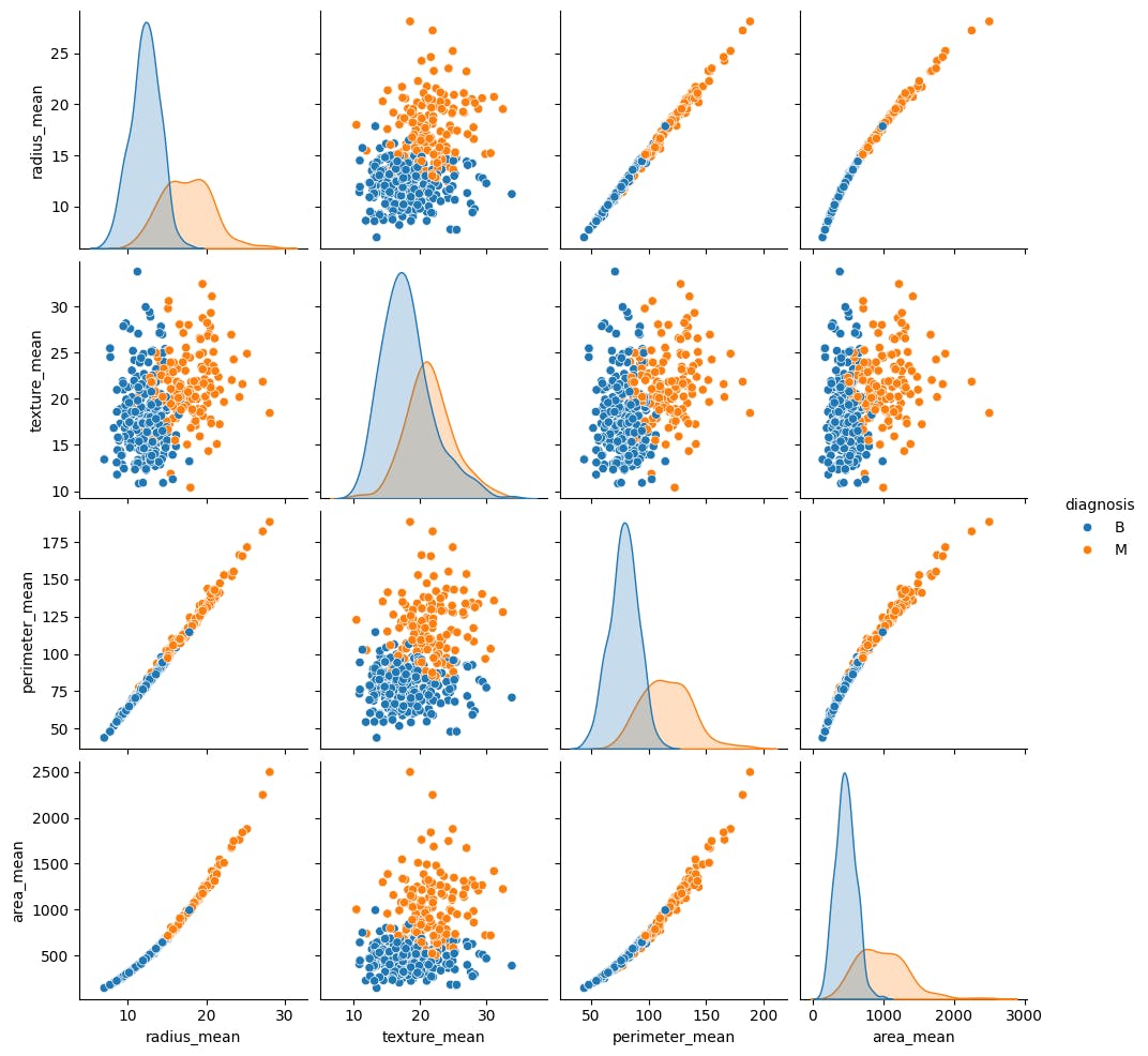
Использоватьseaborn.pairplotЧтобы просмотреть совместное распределение нескольких пар средних функций из учебного набора и наблюдать, как они относятся к цели:

sns.pairplot(train_dataset.iloc[:, 1:6], hue = 'diagnosis', diag_kind='kde');

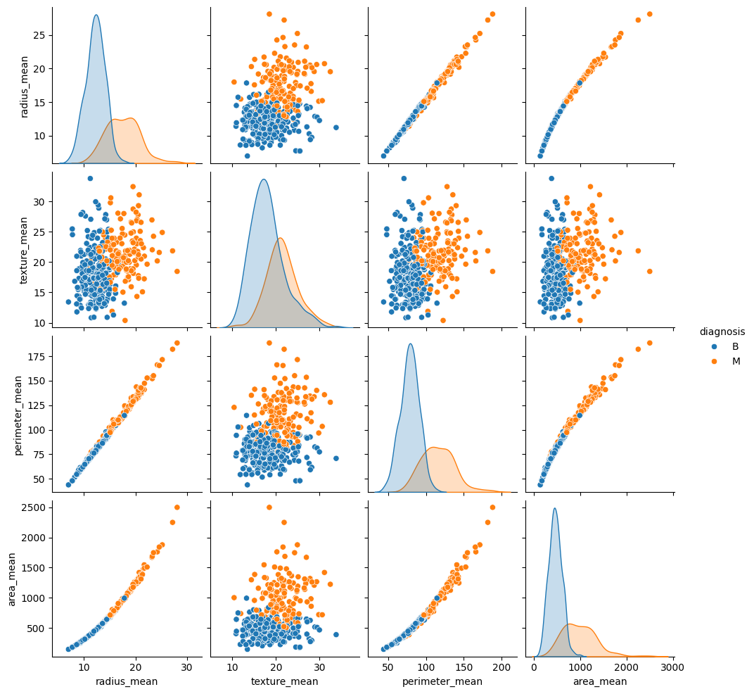
Этот пары демонстрирует, что некоторые особенности, такие как радиус, периметр и область, сильно коррелируют. Это ожидается, так как радиус опухоли непосредственно участвует в вычислении как периметра, так и области. Кроме того, обратите внимание, что злокачественные диагнозы кажутся более правыми для многих функций.

Обязательно проверьте общую статистику. Обратите внимание, как каждая функция охватывает совершенно другой диапазон значений.

train_dataset.describe().transpose()[:10]

Учитывая противоречивые диапазоны, полезно стандартизировать данные, так что каждая функция имеет ноль среднее значение и дисперсию единиц. Этот процесс называетсянормализацияПолем

class Normalize(tf.Module):
  def __init__(self, x):
    # Initialize the mean and standard deviation for normalization
    self.mean = tf.Variable(tf.math.reduce_mean(x, axis=0))
    self.std = tf.Variable(tf.math.reduce_std(x, axis=0))

  def norm(self, x):
    # Normalize the input
    return (x - self.mean)/self.std

  def unnorm(self, x):
    # Unnormalize the input
    return (x * self.std) + self.mean

norm_x = Normalize(x_train)
x_train_norm, x_test_norm = norm_x.norm(x_train), norm_x.norm(x_test)

Логистическая регрессия

Перед созданием модели логистической регрессии крайне важно понять различия метода по сравнению с традиционной линейной регрессией.

Основы логистической регрессии

Линейная регрессия возвращает линейную комбинацию своих входов; Этот вывод неограничен. Выводлогистическая регрессиянаходится в(0, 1)диапазон. Для каждого примера он представляет вероятность того, что пример принадлежитположительныйсорт.

Логистическая регрессия отображает непрерывные результаты традиционной линейной регрессии,(-∞, ∞), вероятно,(0, 1)Полем Это преобразование также является симметричным, так что переворачивание знака линейного выхода приводит к обратному исходному вероятности.

Пусть y обозначает вероятность быть в классе1(опухоль злокачественная). Желаемое отображение может быть достигнуто путем интерпретации вывода линейной регрессии какЖурнал шансовСоотношение в классе1в отличие от класса0:

ln⁡ (y1 -y) = wx+b

Настройка wx+b = z, это уравнение может быть решено для y:

Y = ez1+ez = 11+e - z

Выражение 11+e - z известно каксигмоидальная функцияσ (z). Следовательно, уравнение для логистической регрессии может быть записано как y = σ (wx+b).

Набор данных в этом учебном пособии посвящен высокомерной матрице функции. Следовательно, приведенное выше уравнение должно быть переписано в матричной векторной форме следующим образом:

Y = σ (xw+b)

где:

• YM × 1: целевой вектор
• XM × N: матрица функции
• wn × 1: вектор веса
• b: a bias
• σ: сигмоидальная функция, применяемая к каждому элементу выходного вектора

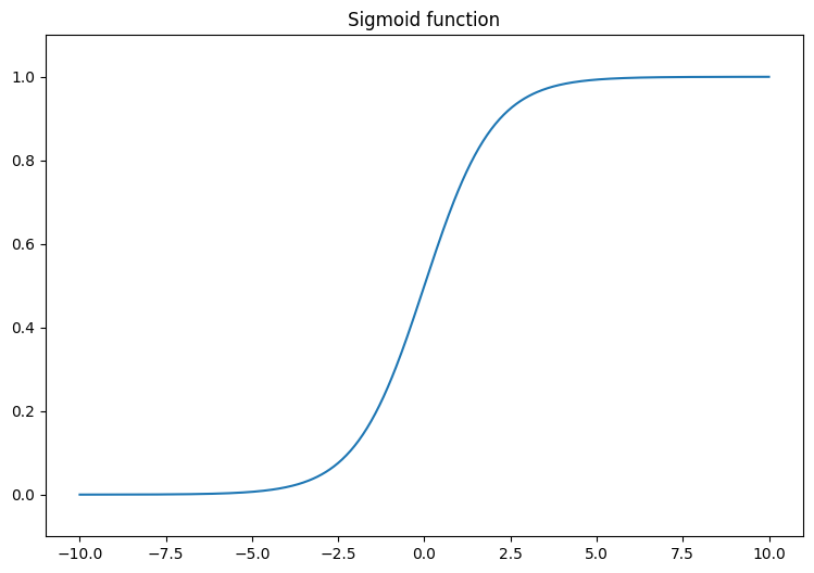
Начните с визуализации сигмоидной функции, которая преобразует линейный выход,(-∞, ∞), чтобы упасть между0и1Полем Сигмовидная функция доступна вtf.math.sigmoidПолем

x = tf.linspace(-10, 10, 500)
x = tf.cast(x, tf.float32)
f = lambda x : (1/20)*x + 0.6
plt.plot(x, tf.math.sigmoid(x))
plt.ylim((-0.1,1.1))
plt.title("Sigmoid function");

Функция потери журнала

АПотеря, или бинарная потери перекрестной энтропии, является идеальной функцией потерь для бинарной задачи классификации с логистической регрессией. Для каждого примера потеря журнала количественно определяет сходство между прогнозируемой вероятностью и истинным значением примера. Это определяется следующим уравнением:

L = −1m∑i = 1myi= log⁡ (y^i)+(1 -yi) Ϫlog⁡ (1 -y^i)

где:

• y^: вектор прогнозируемых вероятностей
• Y: вектор истинных целей

Вы можете использоватьtf.nn.sigmoid_cross_entropy_with_logitsФункция для вычисления потери журнала. Эта функция автоматически применяет активацию сигмоида к выходу регрессии:

def log_loss(y_pred, y):
  # Compute the log loss function
  ce = tf.nn.sigmoid_cross_entropy_with_logits(labels=y, logits=y_pred)
  return tf.reduce_mean(ce)

Правило обновления градиентного спуска

API -интерфейсы TensorFlow Core поддерживают автоматическую дифференциацию сtf.GradientTapeПолем Если вам интересно с математикой, стоящей за логистической регрессиейградиентные обновления, вот краткое объяснение:

В приведенном выше уравнении для потери журнала напомните, что каждый y^i может быть переписан в терминах входов как σ (xiw+b).

Цель состоит в том, чтобы найти w ∗ и b ∗, которые минимизируют потерю журнала:

L = −1m∑i = 1myiig⋅log⁡ (σ (xiw+b))+(1 -yi) ⋅log⁡ (1 - σ (xiw+b))

Принимая градиент L по отношению к W, вы получаете следующее:

∂l∂w = 1m (σ (xw+b) −y) x

Принимая градиент L по отношению к B, вы получаете следующее:

∂l∂b = 1m∑i = 1mσ (xiw+b) −yi

Теперь постройте модель логистической регрессии.

class LogisticRegression(tf.Module):

  def __init__(self):
    self.built = False

  def __call__(self, x, train=True):
    # Initialize the model parameters on the first call
    if not self.built:
      # Randomly generate the weights and the bias term
      rand_w = tf.random.uniform(shape=[x.shape[-1], 1], seed=22)
      rand_b = tf.random.uniform(shape=[], seed=22)
      self.w = tf.Variable(rand_w)
      self.b = tf.Variable(rand_b)
      self.built = True
    # Compute the model output
    z = tf.add(tf.matmul(x, self.w), self.b)
    z = tf.squeeze(z, axis=1)
    if train:
      return z
    return tf.sigmoid(z)

Чтобы подтвердить, убедитесь, что не подготовленная модель выводит значения в диапазоне(0, 1)Для небольшого подмножества обучающих данных.

log_reg = LogisticRegression()

y_pred = log_reg(x_train_norm[:5], train=False)
y_pred.numpy()

array([0.9994985 , 0.9978607 , 0.29620072, 0.01979049, 0.3314926 ],
      dtype=float32)

Затем напишите функцию точности, чтобы вычислить долю правильных классификаций во время обучения. Чтобы получить классификации из прогнозируемых вероятностей, установите порог, для которого все вероятности выше порога принадлежат классу1Полем Это настраиваемый гиперпараметт, который можно установить на0.5как дефолт.

def predict_class(y_pred, thresh=0.5):
  # Return a tensor with  `1` if `y_pred` > `0.5`, and `0` otherwise
  return tf.cast(y_pred > thresh, tf.float32)

def accuracy(y_pred, y):
  # Return the proportion of matches between `y_pred` and `y`
  y_pred = tf.math.sigmoid(y_pred)
  y_pred_class = predict_class(y_pred)
  check_equal = tf.cast(y_pred_class == y,tf.float32)
  acc_val = tf.reduce_mean(check_equal)
  return acc_val

Тренировать модель

Использование мини-партий для обучения обеспечивает как эффективность памяти, так и более высокую конвергенцию. Аtf.data.DatasetAPI имеет полезные функции для партии и перетасовки. API позволяет создавать сложные входные трубопроводы из простых, многоразовых кусочков.

batch_size = 64
train_dataset = tf.data.Dataset.from_tensor_slices((x_train_norm, y_train))
train_dataset = train_dataset.shuffle(buffer_size=x_train.shape[0]).batch(batch_size)
test_dataset = tf.data.Dataset.from_tensor_slices((x_test_norm, y_test))
test_dataset = test_dataset.shuffle(buffer_size=x_test.shape[0]).batch(batch_size)

Теперь напишите петлю обучения для модели логистической регрессии. Цикл использует функцию потери журнала и ее градиенты в отношении ввода, чтобы итеративно обновить параметры модели.

# Set training parameters
epochs = 200
learning_rate = 0.01
train_losses, test_losses = [], []
train_accs, test_accs = [], []

# Set up the training loop and begin training
for epoch in range(epochs):
  batch_losses_train, batch_accs_train = [], []
  batch_losses_test, batch_accs_test = [], []

  # Iterate over the training data
  for x_batch, y_batch in train_dataset:
    with tf.GradientTape() as tape:
      y_pred_batch = log_reg(x_batch)
      batch_loss = log_loss(y_pred_batch, y_batch)
    batch_acc = accuracy(y_pred_batch, y_batch)
    # Update the parameters with respect to the gradient calculations
    grads = tape.gradient(batch_loss, log_reg.variables)
    for g,v in zip(grads, log_reg.variables):
      v.assign_sub(learning_rate * g)
    # Keep track of batch-level training performance
    batch_losses_train.append(batch_loss)
    batch_accs_train.append(batch_acc)

  # Iterate over the testing data
  for x_batch, y_batch in test_dataset:
    y_pred_batch = log_reg(x_batch)
    batch_loss = log_loss(y_pred_batch, y_batch)
    batch_acc = accuracy(y_pred_batch, y_batch)
    # Keep track of batch-level testing performance
    batch_losses_test.append(batch_loss)
    batch_accs_test.append(batch_acc)

  # Keep track of epoch-level model performance
  train_loss, train_acc = tf.reduce_mean(batch_losses_train), tf.reduce_mean(batch_accs_train)
  test_loss, test_acc = tf.reduce_mean(batch_losses_test), tf.reduce_mean(batch_accs_test)
  train_losses.append(train_loss)
  train_accs.append(train_acc)
  test_losses.append(test_loss)
  test_accs.append(test_acc)
  if epoch % 20 == 0:
    print(f"Epoch: {epoch}, Training log loss: {train_loss:.3f}")

Epoch: 0, Training log loss: 0.661
Epoch: 20, Training log loss: 0.418
Epoch: 40, Training log loss: 0.269
Epoch: 60, Training log loss: 0.178
Epoch: 80, Training log loss: 0.137
Epoch: 100, Training log loss: 0.116
Epoch: 120, Training log loss: 0.106
Epoch: 140, Training log loss: 0.096
Epoch: 160, Training log loss: 0.094
Epoch: 180, Training log loss: 0.089

Оценка эффективности

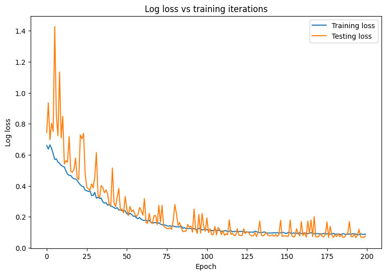
Соблюдайте изменения в потере и точении вашей модели с течением времени.

plt.plot(range(epochs), train_losses, label = "Training loss")
plt.plot(range(epochs), test_losses, label = "Testing loss")
plt.xlabel("Epoch")
plt.ylabel("Log loss")
plt.legend()
plt.title("Log loss vs training iterations");

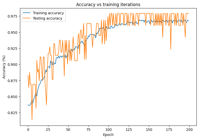
plt.plot(range(epochs), train_accs, label = "Training accuracy")
plt.plot(range(epochs), test_accs, label = "Testing accuracy")
plt.xlabel("Epoch")
plt.ylabel("Accuracy (%)")
plt.legend()
plt.title("Accuracy vs training iterations");

print(f"Final training log loss: {train_losses[-1]:.3f}")
print(f"Final testing log Loss: {test_losses[-1]:.3f}")

Final training log loss: 0.089
Final testing log Loss: 0.077

print(f"Final training accuracy: {train_accs[-1]:.3f}")
print(f"Final testing accuracy: {test_accs[-1]:.3f}")

Final training accuracy: 0.968
Final testing accuracy: 0.979

Модель демонстрирует высокую точность и низкую потерю, когда речь идет о классификации опухолей в учебном наборе данных, а также хорошо обобщает невидимые тестовые данные. Чтобы пойти на шаг вперед, вы можете изучить частоту ошибок, которые дают больше понимания за пределами общей оценки точности. Двумя наиболее популярными частотами ошибок для проблем бинарной классификации являются ложная положительная скорость (FPR) и ложная отрицательная скорость (FNR).

Для этой проблемы FPR - доля прогнозов злокачественных опухолей среди опухолей, которые на самом деле являются доброкачественными. И наоборот, FNR - это доля доброкачественных прогнозов опухолей среди опухолей, которые фактически являются злокачественными.

Вычислить матрицу путаницы, используяsklearn.metrics.confusion_matrix, который оценивает точность классификации и используйте Matplotlib для отображения матрицы:

def show_confusion_matrix(y, y_classes, typ):
  # Compute the confusion matrix and normalize it
  plt.figure(figsize=(10,10))
  confusion = sk_metrics.confusion_matrix(y.numpy(), y_classes.numpy())
  confusion_normalized = confusion / confusion.sum(axis=1, keepdims=True)
  axis_labels = range(2)
  ax = sns.heatmap(
      confusion_normalized, xticklabels=axis_labels, yticklabels=axis_labels,
      cmap='Blues', annot=True, fmt='.4f', square=True)
  plt.title(f"Confusion matrix: {typ}")
  plt.ylabel("True label")
  plt.xlabel("Predicted label")

y_pred_train, y_pred_test = log_reg(x_train_norm, train=False), log_reg(x_test_norm, train=False)
train_classes, test_classes = predict_class(y_pred_train), predict_class(y_pred_test)

show_confusion_matrix(y_train, train_classes, 'Training')

show_confusion_matrix(y_test, test_classes, 'Testing')

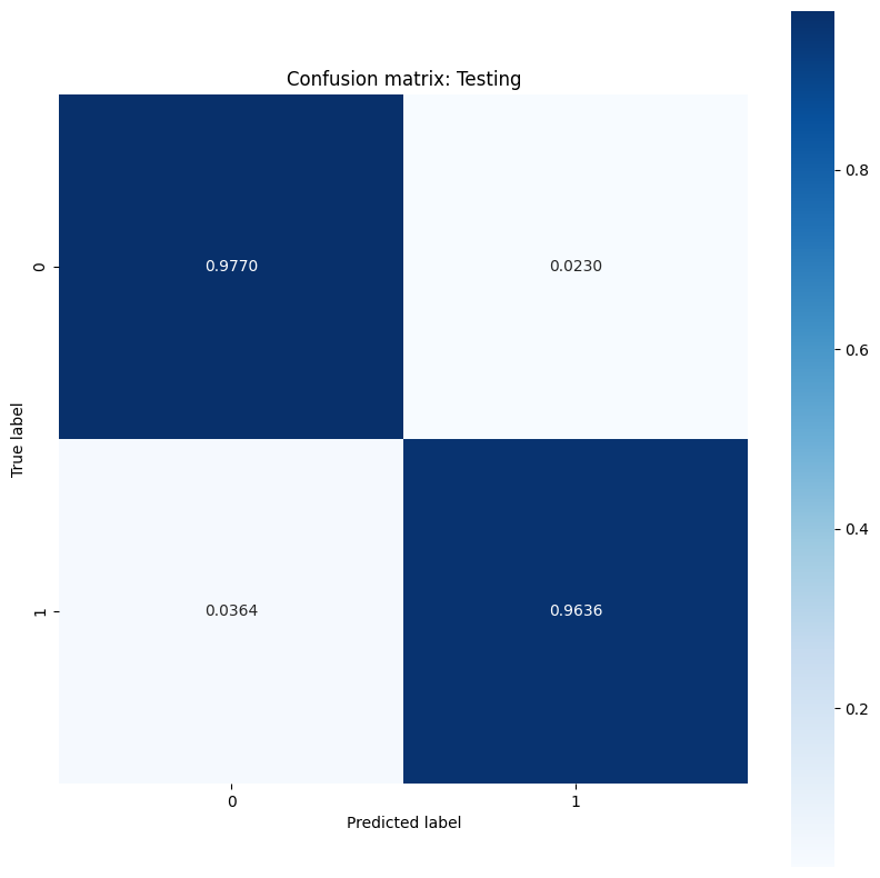
Наблюдайте за измерениями частоты ошибок и интерпретируйте их значение в контексте этого примера. Во многих исследованиях медицинского тестирования, таких как обнаружение рака, высокая ложная положительная частота, чтобы обеспечить низкую ложную негативную частоту вполне приемлемой и фактически поощряется, поскольку риск отсутствия диагноза злокачественной опухоли (ложный отрицательный) намного хуже, чем неправильно классифицировать доброкачественную опухоль как злокачественную (ложную положительную).

Чтобы контролировать FPR и FNR, попробуйте изменить пороговый гиперпараметр, прежде чем классифицировать прогнозы вероятности. Более низкий порог увеличивает общие шансы модели сделать классификацию злокачественных опухолей. Это неизбежно увеличивает количество ложных срабатываний и FPR, но также помогает уменьшить количество ложных отрицательных и FNR.

Сохраните модель

Начните с создания экспортного модуля, который принимает необработанные данные и выполняет следующие операции:

• Нормализация
• Прогнозирование вероятности
• Классовое прогноз

class ExportModule(tf.Module):
  def __init__(self, model, norm_x, class_pred):
    # Initialize pre- and post-processing functions
    self.model = model
    self.norm_x = norm_x
    self.class_pred = class_pred

  @tf.function(input_signature=[tf.TensorSpec(shape=[None, None], dtype=tf.float32)])
  def __call__(self, x):
    # Run the `ExportModule` for new data points
    x = self.norm_x.norm(x)
    y = self.model(x, train=False)
    y = self.class_pred(y)
    return y

log_reg_export = ExportModule(model=log_reg,
                              norm_x=norm_x,
                              class_pred=predict_class)

Если вы хотите сохранить модель в ее текущем состоянии, вы можете сделать это сtf.saved_model.saveфункция Чтобы загрузить сохраненную модель и сделать прогнозы, используйтеtf.saved_model.loadфункция

models = tempfile.mkdtemp()
save_path = os.path.join(models, 'log_reg_export')
tf.saved_model.save(log_reg_export, save_path)

INFO:tensorflow:Assets written to: /tmpfs/tmp/tmp9k_sar52/log_reg_export/assets
INFO:tensorflow:Assets written to: /tmpfs/tmp/tmp9k_sar52/log_reg_export/assets

log_reg_loaded = tf.saved_model.load(save_path)
test_preds = log_reg_loaded(x_test)
test_preds[:10].numpy()

array([1., 1., 1., 1., 0., 1., 1., 1., 1., 1.], dtype=float32)

Заключение

В этом записном книжке было представлено несколько методов для решения проблемы логистической регрессии. Вот еще несколько советов, которые могут помочь:

• АTensorflow Core APIможно использовать для создания рабочих процессов машинного обучения с высоким уровнем конфигурации
• Анализ частоты ошибок - отличный способ получить большее представление о производительности классификации модели за пределами общей оценки точности.
• Персидку - еще одна распространенная проблема для моделей логистической регрессии, хотя это не было проблемой для этого урока. ПосетитьПереоценка и недостатокУчебник для получения дополнительной помощи с этим.

Для получения дополнительных примеров использования API -интерфейсов Core TensorFlow, ознакомьтесь сгидПолем Если вы хотите узнать больше о загрузке и подготовке данных, см. Учебные пособия наЗагрузка данных изображенияилиЗагрузка данных CSVПолем