Оптимизация моделей машинного обучения с точным управлением градиентом в Tensorflow

Обзор контента

• Настраивать
• Контроль градиентной записи
• Прекратить запись
• Сбросить/начать запись с нуля
• Остановить градиент с точностью
• Пользовательские градиенты
• Пользовательские градиенты в SavedModel
• Несколько лент
• Градиенты высшего порядка
• Якобианцы
• Скалярное источник
• Тензор Источник
• Партия якобиан

АВведение в градиенты и автоматическая дифференциацияРуководство включает в себя все, что необходимо для расчета градиентов в TensorFlow. Это руководство фокусируется на более глубоких, менее распространенных чертахtf.GradientTapeAPI.

Настраивать

import tensorflow as tf

import matplotlib as mpl
import matplotlib.pyplot as plt

mpl.rcParams['figure.figsize'] = (8, 6)

2024-08-15 02:32:10.761137: E external/local_xla/xla/stream_executor/cuda/cuda_fft.cc:485] Unable to register cuFFT factory: Attempting to register factory for plugin cuFFT when one has already been registered
2024-08-15 02:32:10.782161: E external/local_xla/xla/stream_executor/cuda/cuda_dnn.cc:8454] Unable to register cuDNN factory: Attempting to register factory for plugin cuDNN when one has already been registered
2024-08-15 02:32:10.788607: E external/local_xla/xla/stream_executor/cuda/cuda_blas.cc:1452] Unable to register cuBLAS factory: Attempting to register factory for plugin cuBLAS when one has already been registered

Контроль градиентной записи

ВРуководство по автоматической дифференциацииВы видели, как контролировать, какие переменные и тензоры наблюдаются лентой при создании расчета градиента.

Лента также имеет методы манипулирования записи.

Прекратить запись

Если вы хотите прекратить записи градиентов, вы можете использоватьtf.GradientTape.stop_recordingвременно приостановить запись.

Это может быть полезно для уменьшения накладных расходов, если вы не хотите дифференцировать сложную операцию в середине вашей модели. Это может включать в себя расчет метрики или промежуточный результат:

x = tf.Variable(2.0)
y = tf.Variable(3.0)

with tf.GradientTape() as t:
  x_sq = x * x
  with t.stop_recording():
    y_sq = y * y
  z = x_sq + y_sq

grad = t.gradient(z, {'x': x, 'y': y})

print('dz/dx:', grad['x'])  # 2*x => 4
print('dz/dy:', grad['y'])

dz/dx: tf.Tensor(4.0, shape=(), dtype=float32)
dz/dy: None
WARNING: All log messages before absl::InitializeLog() is called are written to STDERR
I0000 00:00:1723689133.642575  116670 cuda_executor.cc:1015] successful NUMA node read from SysFS had negative value (-1), but there must be at least one NUMA node, so returning NUMA node zero. See more at https://github.com/torvalds/linux/blob/v6.0/Documentation/ABI/testing/sysfs-bus-pci#L344-L355
I0000 00:00:1723689133.646496  116670 cuda_executor.cc:1015] successful NUMA node read from SysFS had negative value (-1), but there must be at least one NUMA node, so returning NUMA node zero. See more at https://github.com/torvalds/linux/blob/v6.0/Documentation/ABI/testing/sysfs-bus-pci#L344-L355
I0000 00:00:1723689133.650243  116670 cuda_executor.cc:1015] successful NUMA node read from SysFS had negative value (-1), but there must be at least one NUMA node, so returning NUMA node zero. See more at https://github.com/torvalds/linux/blob/v6.0/Documentation/ABI/testing/sysfs-bus-pci#L344-L355
I0000 00:00:1723689133.653354  116670 cuda_executor.cc:1015] successful NUMA node read from SysFS had negative value (-1), but there must be at least one NUMA node, so returning NUMA node zero. See more at https://github.com/torvalds/linux/blob/v6.0/Documentation/ABI/testing/sysfs-bus-pci#L344-L355
I0000 00:00:1723689133.664545  116670 cuda_executor.cc:1015] successful NUMA node read from SysFS had negative value (-1), but there must be at least one NUMA node, so returning NUMA node zero. See more at https://github.com/torvalds/linux/blob/v6.0/Documentation/ABI/testing/sysfs-bus-pci#L344-L355
I0000 00:00:1723689133.668230  116670 cuda_executor.cc:1015] successful NUMA node read from SysFS had negative value (-1), but there must be at least one NUMA node, so returning NUMA node zero. See more at https://github.com/torvalds/linux/blob/v6.0/Documentation/ABI/testing/sysfs-bus-pci#L344-L355
I0000 00:00:1723689133.671627  116670 cuda_executor.cc:1015] successful NUMA node read from SysFS had negative value (-1), but there must be at least one NUMA node, so returning NUMA node zero. See more at https://github.com/torvalds/linux/blob/v6.0/Documentation/ABI/testing/sysfs-bus-pci#L344-L355
I0000 00:00:1723689133.674592  116670 cuda_executor.cc:1015] successful NUMA node read from SysFS had negative value (-1), but there must be at least one NUMA node, so returning NUMA node zero. See more at https://github.com/torvalds/linux/blob/v6.0/Documentation/ABI/testing/sysfs-bus-pci#L344-L355
I0000 00:00:1723689133.677498  116670 cuda_executor.cc:1015] successful NUMA node read from SysFS had negative value (-1), but there must be at least one NUMA node, so returning NUMA node zero. See more at https://github.com/torvalds/linux/blob/v6.0/Documentation/ABI/testing/sysfs-bus-pci#L344-L355
I0000 00:00:1723689133.680982  116670 cuda_executor.cc:1015] successful NUMA node read from SysFS had negative value (-1), but there must be at least one NUMA node, so returning NUMA node zero. See more at https://github.com/torvalds/linux/blob/v6.0/Documentation/ABI/testing/sysfs-bus-pci#L344-L355
I0000 00:00:1723689133.684370  116670 cuda_executor.cc:1015] successful NUMA node read from SysFS had negative value (-1), but there must be at least one NUMA node, so returning NUMA node zero. See more at https://github.com/torvalds/linux/blob/v6.0/Documentation/ABI/testing/sysfs-bus-pci#L344-L355
I0000 00:00:1723689133.687370  116670 cuda_executor.cc:1015] successful NUMA node read from SysFS had negative value (-1), but there must be at least one NUMA node, so returning NUMA node zero. See more at https://github.com/torvalds/linux/blob/v6.0/Documentation/ABI/testing/sysfs-bus-pci#L344-L355
I0000 00:00:1723689134.924735  116670 cuda_executor.cc:1015] successful NUMA node read from SysFS had negative value (-1), but there must be at least one NUMA node, so returning NUMA node zero. See more at https://github.com/torvalds/linux/blob/v6.0/Documentation/ABI/testing/sysfs-bus-pci#L344-L355
I0000 00:00:1723689134.926905  116670 cuda_executor.cc:1015] successful NUMA node read from SysFS had negative value (-1), but there must be at least one NUMA node, so returning NUMA node zero. See more at https://github.com/torvalds/linux/blob/v6.0/Documentation/ABI/testing/sysfs-bus-pci#L344-L355
I0000 00:00:1723689134.928886  116670 cuda_executor.cc:1015] successful NUMA node read from SysFS had negative value (-1), but there must be at least one NUMA node, so returning NUMA node zero. See more at https://github.com/torvalds/linux/blob/v6.0/Documentation/ABI/testing/sysfs-bus-pci#L344-L355
I0000 00:00:1723689134.930883  116670 cuda_executor.cc:1015] successful NUMA node read from SysFS had negative value (-1), but there must be at least one NUMA node, so returning NUMA node zero. See more at https://github.com/torvalds/linux/blob/v6.0/Documentation/ABI/testing/sysfs-bus-pci#L344-L355
I0000 00:00:1723689134.932919  116670 cuda_executor.cc:1015] successful NUMA node read from SysFS had negative value (-1), but there must be at least one NUMA node, so returning NUMA node zero. See more at https://github.com/torvalds/linux/blob/v6.0/Documentation/ABI/testing/sysfs-bus-pci#L344-L355
I0000 00:00:1723689134.934914  116670 cuda_executor.cc:1015] successful NUMA node read from SysFS had negative value (-1), but there must be at least one NUMA node, so returning NUMA node zero. See more at https://github.com/torvalds/linux/blob/v6.0/Documentation/ABI/testing/sysfs-bus-pci#L344-L355
I0000 00:00:1723689134.936798  116670 cuda_executor.cc:1015] successful NUMA node read from SysFS had negative value (-1), but there must be at least one NUMA node, so returning NUMA node zero. See more at https://github.com/torvalds/linux/blob/v6.0/Documentation/ABI/testing/sysfs-bus-pci#L344-L355
I0000 00:00:1723689134.938737  116670 cuda_executor.cc:1015] successful NUMA node read from SysFS had negative value (-1), but there must be at least one NUMA node, so returning NUMA node zero. See more at https://github.com/torvalds/linux/blob/v6.0/Documentation/ABI/testing/sysfs-bus-pci#L344-L355
I0000 00:00:1723689134.940666  116670 cuda_executor.cc:1015] successful NUMA node read from SysFS had negative value (-1), but there must be at least one NUMA node, so returning NUMA node zero. See more at https://github.com/torvalds/linux/blob/v6.0/Documentation/ABI/testing/sysfs-bus-pci#L344-L355
I0000 00:00:1723689134.942634  116670 cuda_executor.cc:1015] successful NUMA node read from SysFS had negative value (-1), but there must be at least one NUMA node, so returning NUMA node zero. See more at https://github.com/torvalds/linux/blob/v6.0/Documentation/ABI/testing/sysfs-bus-pci#L344-L355
I0000 00:00:1723689134.944517  116670 cuda_executor.cc:1015] successful NUMA node read from SysFS had negative value (-1), but there must be at least one NUMA node, so returning NUMA node zero. See more at https://github.com/torvalds/linux/blob/v6.0/Documentation/ABI/testing/sysfs-bus-pci#L344-L355
I0000 00:00:1723689134.946466  116670 cuda_executor.cc:1015] successful NUMA node read from SysFS had negative value (-1), but there must be at least one NUMA node, so returning NUMA node zero. See more at https://github.com/torvalds/linux/blob/v6.0/Documentation/ABI/testing/sysfs-bus-pci#L344-L355
I0000 00:00:1723689134.984712  116670 cuda_executor.cc:1015] successful NUMA node read from SysFS had negative value (-1), but there must be at least one NUMA node, so returning NUMA node zero. See more at https://github.com/torvalds/linux/blob/v6.0/Documentation/ABI/testing/sysfs-bus-pci#L344-L355
I0000 00:00:1723689134.986787  116670 cuda_executor.cc:1015] successful NUMA node read from SysFS had negative value (-1), but there must be at least one NUMA node, so returning NUMA node zero. See more at https://github.com/torvalds/linux/blob/v6.0/Documentation/ABI/testing/sysfs-bus-pci#L344-L355
I0000 00:00:1723689134.988685  116670 cuda_executor.cc:1015] successful NUMA node read from SysFS had negative value (-1), but there must be at least one NUMA node, so returning NUMA node zero. See more at https://github.com/torvalds/linux/blob/v6.0/Documentation/ABI/testing/sysfs-bus-pci#L344-L355
I0000 00:00:1723689134.990637  116670 cuda_executor.cc:1015] successful NUMA node read from SysFS had negative value (-1), but there must be at least one NUMA node, so returning NUMA node zero. See more at https://github.com/torvalds/linux/blob/v6.0/Documentation/ABI/testing/sysfs-bus-pci#L344-L355
I0000 00:00:1723689134.993156  116670 cuda_executor.cc:1015] successful NUMA node read from SysFS had negative value (-1), but there must be at least one NUMA node, so returning NUMA node zero. See more at https://github.com/torvalds/linux/blob/v6.0/Documentation/ABI/testing/sysfs-bus-pci#L344-L355
I0000 00:00:1723689134.995163  116670 cuda_executor.cc:1015] successful NUMA node read from SysFS had negative value (-1), but there must be at least one NUMA node, so returning NUMA node zero. See more at https://github.com/torvalds/linux/blob/v6.0/Documentation/ABI/testing/sysfs-bus-pci#L344-L355
I0000 00:00:1723689134.997026  116670 cuda_executor.cc:1015] successful NUMA node read from SysFS had negative value (-1), but there must be at least one NUMA node, so returning NUMA node zero. See more at https://github.com/torvalds/linux/blob/v6.0/Documentation/ABI/testing/sysfs-bus-pci#L344-L355
I0000 00:00:1723689134.998929  116670 cuda_executor.cc:1015] successful NUMA node read from SysFS had negative value (-1), but there must be at least one NUMA node, so returning NUMA node zero. See more at https://github.com/torvalds/linux/blob/v6.0/Documentation/ABI/testing/sysfs-bus-pci#L344-L355
I0000 00:00:1723689135.000885  116670 cuda_executor.cc:1015] successful NUMA node read from SysFS had negative value (-1), but there must be at least one NUMA node, so returning NUMA node zero. See more at https://github.com/torvalds/linux/blob/v6.0/Documentation/ABI/testing/sysfs-bus-pci#L344-L355
I0000 00:00:1723689135.003378  116670 cuda_executor.cc:1015] successful NUMA node read from SysFS had negative value (-1), but there must be at least one NUMA node, so returning NUMA node zero. See more at https://github.com/torvalds/linux/blob/v6.0/Documentation/ABI/testing/sysfs-bus-pci#L344-L355
I0000 00:00:1723689135.005704  116670 cuda_executor.cc:1015] successful NUMA node read from SysFS had negative value (-1), but there must be at least one NUMA node, so returning NUMA node zero. See more at https://github.com/torvalds/linux/blob/v6.0/Documentation/ABI/testing/sysfs-bus-pci#L344-L355
I0000 00:00:1723689135.008045  116670 cuda_executor.cc:1015] successful NUMA node read from SysFS had negative value (-1), but there must be at least one NUMA node, so returning NUMA node zero. See more at https://github.com/torvalds/linux/blob/v6.0/Documentation/ABI/testing/sysfs-bus-pci#L344-L355

Сбросить/начать запись с нуля

Если вы хотите начать полностью, используйтеtf.GradientTape.resetПолем Просто выходить из градиентного ленточного блока и перезагрузки, как правило, легче читать, но вы можете использоватьresetМетод при выходе из ленточного блока сложно или невозможно.

x = tf.Variable(2.0)
y = tf.Variable(3.0)
reset = True

with tf.GradientTape() as t:
  y_sq = y * y
  if reset:
    # Throw out all the tape recorded so far.
    t.reset()
  z = x * x + y_sq

grad = t.gradient(z, {'x': x, 'y': y})

print('dz/dx:', grad['x'])  # 2*x => 4
print('dz/dy:', grad['y'])

dz/dx: tf.Tensor(4.0, shape=(), dtype=float32)
dz/dy: None

Остановить градиент с точностью

В отличие от глобальных элементов управления лентой, вышеtf.stop_gradientФункция гораздо точнее. Его можно использовать, чтобы помешать градиентам течь по конкретному пути, не требуя доступа к самой ленте:

x = tf.Variable(2.0)
y = tf.Variable(3.0)

with tf.GradientTape() as t:
  y_sq = y**2
  z = x**2 + tf.stop_gradient(y_sq)

grad = t.gradient(z, {'x': x, 'y': y})

print('dz/dx:', grad['x'])  # 2*x => 4
print('dz/dy:', grad['y'])

dz/dx: tf.Tensor(4.0, shape=(), dtype=float32)
dz/dy: None

Пользовательские градиенты

В некоторых случаях вы можете контролировать, как именно рассчитываются градиенты, а не использовать дефолт. Эти ситуации включают:

1. Нет определенного градиента для нового OP, который вы пишете.
2. Расчеты по умолчанию численно нестабильны.
3. Вы хотите кэшировать дорогостоящие вычисления из прямого прохода.
4. Вы хотите изменить значение (например, используяtf.clip_by_valueилиtf.math.round) без изменения градиента.

Для первого случая написать новый OP, который вы можете использоватьtf.RegisterGradientЧтобы настроить свои собственные (см. Документы API для получения подробной информации). (Обратите внимание, что градиентный реестр является глобальным, поэтому измените его с осторожностью.)

Для последних трех случаев вы можете использоватьtf.custom_gradientПолем

Вот пример, который применяетсяtf.clip_by_normк промежуточному градиенту:

# Establish an identity operation, but clip during the gradient pass.
@tf.custom_gradient
def clip_gradients(y):
  def backward(dy):
    return tf.clip_by_norm(dy, 0.5)
  return y, backward

v = tf.Variable(2.0)
with tf.GradientTape() as t:
  output = clip_gradients(v * v)
print(t.gradient(output, v))  # calls "backward", which clips 4 to 2

tf.Tensor(2.0, shape=(), dtype=float32)

Смtf.custom_gradientДекоратор API DOCS для более подробной информации.

Пользовательские градиенты в SavedModel

Пользовательские градиенты могут быть сохранены в SavedModel с помощью опцииtf.saved_model.SaveOptions(experimental_custom_gradients=True)Полем

Чтобы сохранить в сохранении модели, функция градиента должна быть отслеживаемой (чтобы узнать больше, ознакомьтесь сЛучшая производительность с tf.functionгид).

class MyModule(tf.Module):

  @tf.function(input_signature=[tf.TensorSpec(None)])
  def call_custom_grad(self, x):
    return clip_gradients(x)

model = MyModule()

tf.saved_model.save(
    model,
    'saved_model',
    options=tf.saved_model.SaveOptions(experimental_custom_gradients=True))

# The loaded gradients will be the same as the above example.
v = tf.Variable(2.0)
loaded = tf.saved_model.load('saved_model')
with tf.GradientTape() as t:
  output = loaded.call_custom_grad(v * v)
print(t.gradient(output, v))

INFO:tensorflow:Assets written to: saved_model/assets
INFO:tensorflow:Assets written to: saved_model/assets
tf.Tensor(2.0, shape=(), dtype=float32)

Примечание о приведенном выше примере: если вы попытаетесь заменить приведенный выше кодtf.saved_model.SaveOptions(experimental_custom_gradients=False), градиент по -прежнему даст тот же результат при загрузке. Причина в том, что градиентный реестр по -прежнему содержит пользовательский градиент, используемый в функцииcall_custom_opПолем Однако, если вы перезапустите время выполнения после сохранения без пользовательских градиентов, запустив загруженную модель подtf.GradientTapeбросит ошибку:LookupError: No gradient defined for operation 'IdentityN' (op type: IdentityN)Полем

Несколько лент

Несколько лент беспрепятственно взаимодействуют.

Например, здесь каждая лента наблюдает за различным набором тензоров:

x0 = tf.constant(0.0)
x1 = tf.constant(0.0)

with tf.GradientTape() as tape0, tf.GradientTape() as tape1:
  tape0.watch(x0)
  tape1.watch(x1)

  y0 = tf.math.sin(x0)
  y1 = tf.nn.sigmoid(x1)

  y = y0 + y1

  ys = tf.reduce_sum(y)

tape0.gradient(ys, x0).numpy()   # cos(x) => 1.0

1.0

tape1.gradient(ys, x1).numpy()   # sigmoid(x1)*(1-sigmoid(x1)) => 0.25

0.25

Градиенты высшего порядка

Операции внутриtf.GradientTapeКонтекст -менеджер записывается для автоматической дифференциации. Если в этом контексте вычисляются градиенты, то вычисление градиента также записывается. В результате тот же API работает и для градиентов высшего порядка.

Например:

x = tf.Variable(1.0)  # Create a Tensorflow variable initialized to 1.0

with tf.GradientTape() as t2:
  with tf.GradientTape() as t1:
    y = x * x * x

  # Compute the gradient inside the outer `t2` context manager
  # which means the gradient computation is differentiable as well.
  dy_dx = t1.gradient(y, x)
d2y_dx2 = t2.gradient(dy_dx, x)

print('dy_dx:', dy_dx.numpy())  # 3 * x**2 => 3.0
print('d2y_dx2:', d2y_dx2.numpy())  # 6 * x => 6.0

dy_dx: 3.0
d2y_dx2: 6.0

Хотя это дает вам вторую производнуюСкалярфункция, этот шаблон не обобщается для создания гесстской матрицы, посколькуtf.GradientTape.gradientТолько вычисляет градиент скаляр. Построить аГессианская матрица, пойти вГессианский примерподЯкобианская секцияПолем

"Вложенные звонкиtf.GradientTape.gradient«Это хорошая схема, когда вы расчет скаляр из градиента, а затем полученные скалярные действия действуют в качестве источника для второго расчета градиента, как в следующем примере.

Пример: регуляризация ввода градиента

Многие модели восприимчивы к «состязательным примерам». Эта коллекция методов изменяет вход модели, чтобы запутать вывод модели. Самая простая реализация, напримерПример состязания с использованием атаки метода быстрого градиента- выполняет один шаг вдоль градиента выхода по отношению к входу; «входной градиент».

Одним из методов повышения устойчивости к состязательным примерам являетсяВходной градиент регуляризация(Finlay & Oberman, 2019), который пытается минимизировать величину входного градиента. Если входной градиент невелик, то изменение выхода также должно быть небольшим.

Ниже приведена наивная реализация регуляризации входного градиента. Реализация:

1. Рассчитайте градиент вывода относительно входа, используя внутреннюю ленту.
2. Рассчитайте величину этого входного градиента.
3. Рассчитайте градиент такого масштаба относительно модели.

x = tf.random.normal([7, 5])

layer = tf.keras.layers.Dense(10, activation=tf.nn.relu)

with tf.GradientTape() as t2:
  # The inner tape only takes the gradient with respect to the input,
  # not the variables.
  with tf.GradientTape(watch_accessed_variables=False) as t1:
    t1.watch(x)
    y = layer(x)
    out = tf.reduce_sum(layer(x)**2)
  # 1. Calculate the input gradient.
  g1 = t1.gradient(out, x)
  # 2. Calculate the magnitude of the input gradient.
  g1_mag = tf.norm(g1)

# 3. Calculate the gradient of the magnitude with respect to the model.
dg1_mag = t2.gradient(g1_mag, layer.trainable_variables)

[var.shape for var in dg1_mag]

[TensorShape([5, 10]), TensorShape([10])]

Якобианцы

Все предыдущие примеры взяли градиенты скалярной цели в отношении некоторых тензоров (ах) источника.

АЯкобианская матрицапредставляет градиенты векторной оцененной функции. Каждый ряд содержит градиент одного из элементов вектора.

Аtf.GradientTape.jacobianМетод позволяет эффективно рассчитать якобийскую матрицу.

Обратите внимание, что:

• Нравитьсяgradient:sourcesАргумент может быть тензором или контейнером из тензоров.
• В отличие отgradient:targetТензор должен быть единственным тензором.

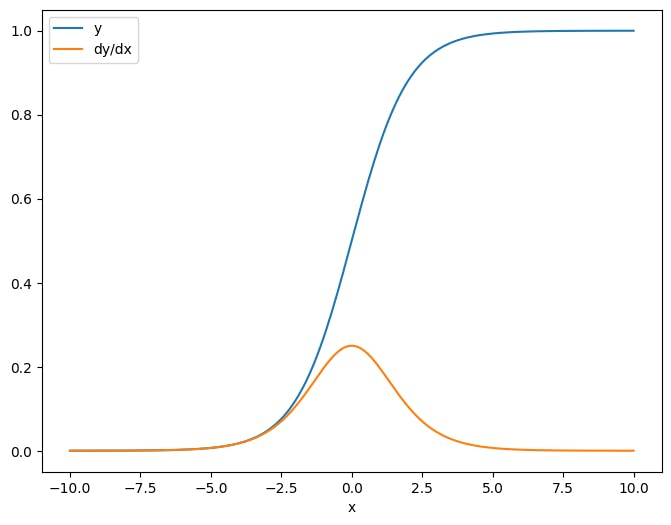
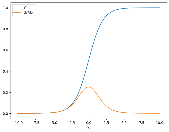
Скалярное источник

В качестве первого примера, вот якобийский вектор-мишень относительно скалярного источника.

x = tf.linspace(-10.0, 10.0, 200+1)
delta = tf.Variable(0.0)

with tf.GradientTape() as tape:
  y = tf.nn.sigmoid(x+delta)

dy_dx = tape.jacobian(y, delta)

Когда вы берете якобиан по отношению к скаляр, результат имеет формуцельи дает градиент каждого элемента относительно источника:

print(y.shape)
print(dy_dx.shape)

(201,)
(201,)

plt.plot(x.numpy(), y, label='y')
plt.plot(x.numpy(), dy_dx, label='dy/dx')
plt.legend()
_ = plt.xlabel('x')

Тензор Источник

Будь то вход скалярным или тензором,tf.GradientTape.jacobianЭффективно рассчитывает градиент каждого элемента источника по отношению к каждому элементу цели.

Например, выход этого слоя имеет форму(10, 7):

x = tf.random.normal([7, 5])
layer = tf.keras.layers.Dense(10, activation=tf.nn.relu)

with tf.GradientTape(persistent=True) as tape:
  y = layer(x)

y.shape

TensorShape([7, 10])

И форма ядра слоя(5, 10):

layer.kernel.shape

TensorShape([5, 10])

Форма якобиана вывода по отношению к ядру - эти две формы, объединенные вместе:

j = tape.jacobian(y, layer.kernel)
j.shape

TensorShape([7, 10, 5, 10])

Если вы суммируете измерения цели, у вас останется градиент суммы, которая была бы рассчитанаtf.GradientTape.gradient:

g = tape.gradient(y, layer.kernel)
print('g.shape:', g.shape)

j_sum = tf.reduce_sum(j, axis=[0, 1])
delta = tf.reduce_max(abs(g - j_sum)).numpy()
assert delta < 1e-3
print('delta:', delta)

g.shape: (5, 10)
delta: 2.3841858e-07

Пример: Гессиан

Покаtf.GradientTapeне дает явный метод для построенияГессианская матрицаможно построить один, используяtf.GradientTape.jacobianметод

x = tf.random.normal([7, 5])
layer1 = tf.keras.layers.Dense(8, activation=tf.nn.relu)
layer2 = tf.keras.layers.Dense(6, activation=tf.nn.relu)

with tf.GradientTape() as t2:
  with tf.GradientTape() as t1:
    x = layer1(x)
    x = layer2(x)
    loss = tf.reduce_mean(x**2)

  g = t1.gradient(loss, layer1.kernel)

h = t2.jacobian(g, layer1.kernel)

print(f'layer.kernel.shape: {layer1.kernel.shape}')
print(f'h.shape: {h.shape}')

layer.kernel.shape: (5, 8)
h.shape: (5, 8, 5, 8)

Чтобы использовать этот гессиан дляМетод НьютонаШаг, вы сначала выплющили его оси в матрицу и расплющили градиент в вектор:

n_params = tf.reduce_prod(layer1.kernel.shape)

g_vec = tf.reshape(g, [n_params, 1])
h_mat = tf.reshape(h, [n_params, n_params])

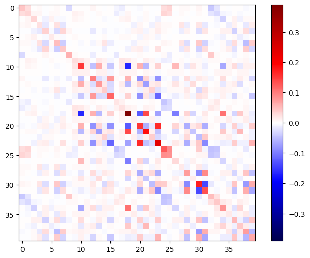
Гессианская матрица должна быть симметричной:

def imshow_zero_center(image, **kwargs):
  lim = tf.reduce_max(abs(image))
  plt.imshow(image, vmin=-lim, vmax=lim, cmap='seismic', **kwargs)
  plt.colorbar()

imshow_zero_center(h_mat)

Шаг обновления метода Ньютона показан ниже:

eps = 1e-3
eye_eps = tf.eye(h_mat.shape[0])*eps

# X(k+1) = X(k) - (∇²f(X(k)))^-1 @ ∇f(X(k))
# h_mat = ∇²f(X(k))
# g_vec = ∇f(X(k))
update = tf.linalg.solve(h_mat + eye_eps, g_vec)

# Reshape the update and apply it to the variable.
_ = layer1.kernel.assign_sub(tf.reshape(update, layer1.kernel.shape))

Хотя это относительно просто для одногоtf.VariableПрименение этого к нетривиальной модели потребует тщательной объединения и нарезки для производства полного гессиана по нескольким переменным.

Партия якобиан

В некоторых случаях вы хотите взять якобиана каждой из целей в отношении стопки источников, где якобианцы для каждой пары-целевого источника являются независимыми.

Например, здесь входxформируется(batch, ins)и выводyформируется(batch, outs):

x = tf.random.normal([7, 5])

layer1 = tf.keras.layers.Dense(8, activation=tf.nn.elu)
layer2 = tf.keras.layers.Dense(6, activation=tf.nn.elu)

with tf.GradientTape(persistent=True, watch_accessed_variables=False) as tape:
  tape.watch(x)
  y = layer1(x)
  y = layer2(y)

y.shape

TensorShape([7, 6])

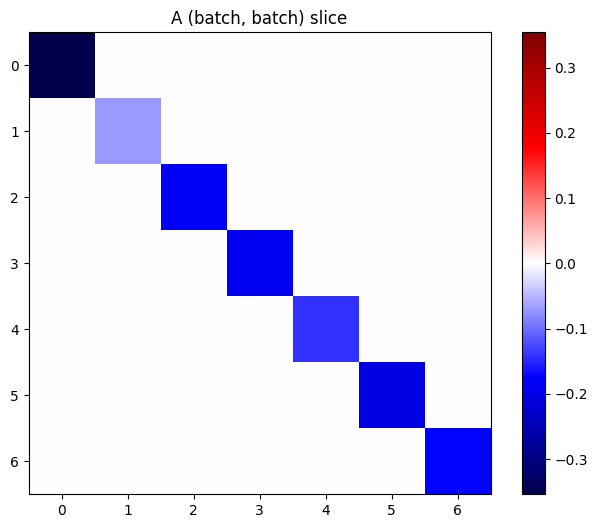
Полный якобианyЧто касаетсяxимеет форму(batch, ins, batch, outs), даже если вы хотите только(batch, ins, outs):

j = tape.jacobian(y, x)
j.shape

TensorShape([7, 6, 7, 5])

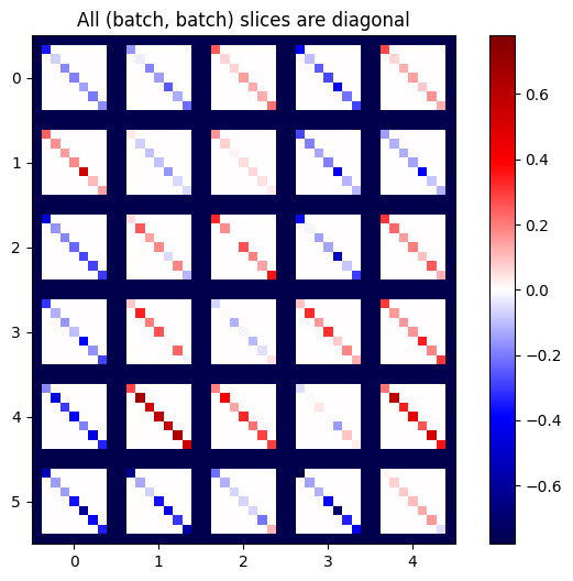
Если градиенты каждого элемента в стеке независимы, то каждый(batch, batch)Ломтик этого тензора - диагональная матрица:

imshow_zero_center(j[:, 0, :, 0])
_ = plt.title('A (batch, batch) slice')

def plot_as_patches(j):
  # Reorder axes so the diagonals will each form a contiguous patch.
  j = tf.transpose(j, [1, 0, 3, 2])
  # Pad in between each patch.
  lim = tf.reduce_max(abs(j))
  j = tf.pad(j, [[0, 0], [1, 1], [0, 0], [1, 1]],
             constant_values=-lim)
  # Reshape to form a single image.
  s = j.shape
  j = tf.reshape(j, [s[0]*s[1], s[2]*s[3]])
  imshow_zero_center(j, extent=[-0.5, s[2]-0.5, s[0]-0.5, -0.5])

plot_as_patches(j)
_ = plt.title('All (batch, batch) slices are diagonal')

Чтобы получить желаемый результат, вы можете подвести итог по дубликатуbatchразмер или выберите диагонали, используяtf.einsum:

j_sum = tf.reduce_sum(j, axis=2)
print(j_sum.shape)
j_select = tf.einsum('bxby->bxy', j)
print(j_select.shape)

(7, 6, 5)
(7, 6, 5)

Было бы гораздо эффективнее выполнить расчет без дополнительного измерения в первую очередь. Аtf.GradientTape.batch_jacobianМетод делает именно это:

jb = tape.batch_jacobian(y, x)
jb.shape

WARNING:tensorflow:5 out of the last 5 calls to <function pfor.<locals>.f at 0x7f968c10d700> triggered tf.function retracing. Tracing is expensive and the excessive number of tracings could be due to (1) creating @tf.function repeatedly in a loop, (2) passing tensors with different shapes, (3) passing Python objects instead of tensors. For (1), please define your @tf.function outside of the loop. For (2), @tf.function has reduce_retracing=True option that can avoid unnecessary retracing. For (3), please refer to https://www.tensorflow.org/guide/function#controlling_retracing and https://www.tensorflow.org/api_docs/python/tf/function for  more details.
WARNING:tensorflow:5 out of the last 5 calls to <function pfor.<locals>.f at 0x7f968c10d700> triggered tf.function retracing. Tracing is expensive and the excessive number of tracings could be due to (1) creating @tf.function repeatedly in a loop, (2) passing tensors with different shapes, (3) passing Python objects instead of tensors. For (1), please define your @tf.function outside of the loop. For (2), @tf.function has reduce_retracing=True option that can avoid unnecessary retracing. For (3), please refer to https://www.tensorflow.org/guide/function#controlling_retracing and https://www.tensorflow.org/api_docs/python/tf/function for  more details.
TensorShape([7, 6, 5])

error = tf.reduce_max(abs(jb - j_sum))
assert error < 1e-3
print(error.numpy())

0.0

x = tf.random.normal([7, 5])

layer1 = tf.keras.layers.Dense(8, activation=tf.nn.elu)
bn = tf.keras.layers.BatchNormalization()
layer2 = tf.keras.layers.Dense(6, activation=tf.nn.elu)

with tf.GradientTape(persistent=True, watch_accessed_variables=False) as tape:
  tape.watch(x)
  y = layer1(x)
  y = bn(y, training=True)
  y = layer2(y)

j = tape.jacobian(y, x)
print(f'j.shape: {j.shape}')

WARNING:tensorflow:6 out of the last 6 calls to <function pfor.<locals>.f at 0x7f967c72d430> triggered tf.function retracing. Tracing is expensive and the excessive number of tracings could be due to (1) creating @tf.function repeatedly in a loop, (2) passing tensors with different shapes, (3) passing Python objects instead of tensors. For (1), please define your @tf.function outside of the loop. For (2), @tf.function has reduce_retracing=True option that can avoid unnecessary retracing. For (3), please refer to https://www.tensorflow.org/guide/function#controlling_retracing and https://www.tensorflow.org/api_docs/python/tf/function for  more details.
WARNING:tensorflow:6 out of the last 6 calls to <function pfor.<locals>.f at 0x7f967c72d430> triggered tf.function retracing. Tracing is expensive and the excessive number of tracings could be due to (1) creating @tf.function repeatedly in a loop, (2) passing tensors with different shapes, (3) passing Python objects instead of tensors. For (1), please define your @tf.function outside of the loop. For (2), @tf.function has reduce_retracing=True option that can avoid unnecessary retracing. For (3), please refer to https://www.tensorflow.org/guide/function#controlling_retracing and https://www.tensorflow.org/api_docs/python/tf/function for  more details.
j.shape: (7, 6, 7, 5)

plot_as_patches(j)

_ = plt.title('These slices are not diagonal')
_ = plt.xlabel("Don't use `batch_jacobian`")

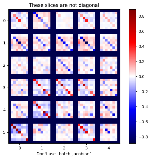
В этом случае,batch_jacobianвсе еще бежит и возвращаетсячто-нибудьс ожидаемой формой, но его содержание имеет неясное значение:

jb = tape.batch_jacobian(y, x)
print(f'jb.shape: {jb.shape}')

jb.shape: (7, 6, 5)