Как сжимать изображения с помощью API SVD и TensorFlow Core

Обзор контента

• Введение
• Настраивать
• Основы SVD
• Низкое приближение ранга с SVD
• Загрузка изображения
• Алгоритм сжатия изображения
• Оценка приближения
• Коэффициент сжатия против ранга
• Кумулятивная сумма единственных значений
• Ошибка и единственные значения
• Заключение

Введение

В этом уроке исследует техникаУниверситетское разложение ценности(SVD) и его приложения для проблем с низким уровнем приближения. SVD используется для факторизации реальных или сложных матриц и имеет различные варианты использования в науке о данных, такие как сжатие изображений. Изображения для этого урока поступают из Google Brain'sВоображениепроект.

Настраивать

import matplotlib
from matplotlib.image import imread
from matplotlib import pyplot as plt
import requests
# Preset Matplotlib figure sizes.
matplotlib.rcParams['figure.figsize'] = [16, 9]

import tensorflow as tf
print(tf.__version__)

2024-08-15 02:40:31.007111: E external/local_xla/xla/stream_executor/cuda/cuda_fft.cc:485] Unable to register cuFFT factory: Attempting to register factory for plugin cuFFT when one has already been registered
2024-08-15 02:40:31.028202: E external/local_xla/xla/stream_executor/cuda/cuda_dnn.cc:8454] Unable to register cuDNN factory: Attempting to register factory for plugin cuDNN when one has already been registered
2024-08-15 02:40:31.034794: E external/local_xla/xla/stream_executor/cuda/cuda_blas.cc:1452] Unable to register cuBLAS factory: Attempting to register factory for plugin cuBLAS when one has already been registered
2.17.0

Основы SVD

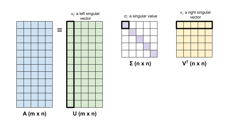
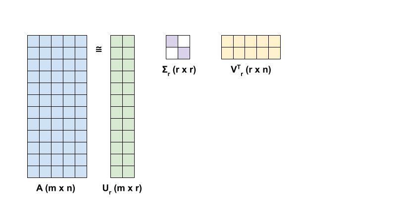
Разложение единственного значения матрицы, а определяется следующей факторизацией:

A = uσvt

где

• Am × N: входная матрица, где m≥n
• Um × n: ортогональная матрица, utu = i, с каждым столбцом, пользовательский интерфейс, обозначающий левый единственный вектор
• Σn × n: диагональная матрица с каждым диагональным входом, σi, обозначающим единственное значение
• Vtn × n: ортогональная матрица, vtv = i, с каждым рядом, vi, обозначающий правый единственный вектор

Когда m <n, U и σ имеют размер (M × M), а VT имеет размер (M × n).

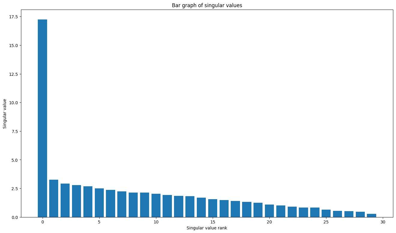
Линейный пакет алгебры Tensorflow имеет функцию,tf.linalg.svd, который может быть использован для вычисления декомпозиции единственного значения одной или нескольких матриц. Начните с определения простой матрицы и вычисления ее факторизации SVD.

A = tf.random.uniform(shape=[40,30])
# Compute the SVD factorization
s, U, V = tf.linalg.svd(A)
# Define Sigma and V Transpose
S = tf.linalg.diag(s)
V_T = tf.transpose(V)
# Reconstruct the original matrix
A_svd = U@S@V_T
# Visualize 
plt.bar(range(len(s)), s);
plt.xlabel("Singular value rank")
plt.ylabel("Singular value")
plt.title("Bar graph of singular values");

WARNING: All log messages before absl::InitializeLog() is called are written to STDERR
I0000 00:00:1723689633.424919  126589 cuda_executor.cc:1015] successful NUMA node read from SysFS had negative value (-1), but there must be at least one NUMA node, so returning NUMA node zero. See more at https://github.com/torvalds/linux/blob/v6.0/Documentation/ABI/testing/sysfs-bus-pci#L344-L355
I0000 00:00:1723689633.428762  126589 cuda_executor.cc:1015] successful NUMA node read from SysFS had negative value (-1), but there must be at least one NUMA node, so returning NUMA node zero. See more at https://github.com/torvalds/linux/blob/v6.0/Documentation/ABI/testing/sysfs-bus-pci#L344-L355
I0000 00:00:1723689633.432420  126589 cuda_executor.cc:1015] successful NUMA node read from SysFS had negative value (-1), but there must be at least one NUMA node, so returning NUMA node zero. See more at https://github.com/torvalds/linux/blob/v6.0/Documentation/ABI/testing/sysfs-bus-pci#L344-L355
I0000 00:00:1723689633.437707  126589 cuda_executor.cc:1015] successful NUMA node read from SysFS had negative value (-1), but there must be at least one NUMA node, so returning NUMA node zero. See more at https://github.com/torvalds/linux/blob/v6.0/Documentation/ABI/testing/sysfs-bus-pci#L344-L355
I0000 00:00:1723689633.449819  126589 cuda_executor.cc:1015] successful NUMA node read from SysFS had negative value (-1), but there must be at least one NUMA node, so returning NUMA node zero. See more at https://github.com/torvalds/linux/blob/v6.0/Documentation/ABI/testing/sysfs-bus-pci#L344-L355
I0000 00:00:1723689633.453529  126589 cuda_executor.cc:1015] successful NUMA node read from SysFS had negative value (-1), but there must be at least one NUMA node, so returning NUMA node zero. See more at https://github.com/torvalds/linux/blob/v6.0/Documentation/ABI/testing/sysfs-bus-pci#L344-L355
I0000 00:00:1723689633.457079  126589 cuda_executor.cc:1015] successful NUMA node read from SysFS had negative value (-1), but there must be at least one NUMA node, so returning NUMA node zero. See more at https://github.com/torvalds/linux/blob/v6.0/Documentation/ABI/testing/sysfs-bus-pci#L344-L355
I0000 00:00:1723689633.460600  126589 cuda_executor.cc:1015] successful NUMA node read from SysFS had negative value (-1), but there must be at least one NUMA node, so returning NUMA node zero. See more at https://github.com/torvalds/linux/blob/v6.0/Documentation/ABI/testing/sysfs-bus-pci#L344-L355
I0000 00:00:1723689633.464019  126589 cuda_executor.cc:1015] successful NUMA node read from SysFS had negative value (-1), but there must be at least one NUMA node, so returning NUMA node zero. See more at https://github.com/torvalds/linux/blob/v6.0/Documentation/ABI/testing/sysfs-bus-pci#L344-L355
I0000 00:00:1723689633.467451  126589 cuda_executor.cc:1015] successful NUMA node read from SysFS had negative value (-1), but there must be at least one NUMA node, so returning NUMA node zero. See more at https://github.com/torvalds/linux/blob/v6.0/Documentation/ABI/testing/sysfs-bus-pci#L344-L355
I0000 00:00:1723689633.470857  126589 cuda_executor.cc:1015] successful NUMA node read from SysFS had negative value (-1), but there must be at least one NUMA node, so returning NUMA node zero. See more at https://github.com/torvalds/linux/blob/v6.0/Documentation/ABI/testing/sysfs-bus-pci#L344-L355
I0000 00:00:1723689633.474376  126589 cuda_executor.cc:1015] successful NUMA node read from SysFS had negative value (-1), but there must be at least one NUMA node, so returning NUMA node zero. See more at https://github.com/torvalds/linux/blob/v6.0/Documentation/ABI/testing/sysfs-bus-pci#L344-L355
I0000 00:00:1723689634.696864  126589 cuda_executor.cc:1015] successful NUMA node read from SysFS had negative value (-1), but there must be at least one NUMA node, so returning NUMA node zero. See more at https://github.com/torvalds/linux/blob/v6.0/Documentation/ABI/testing/sysfs-bus-pci#L344-L355
I0000 00:00:1723689634.698995  126589 cuda_executor.cc:1015] successful NUMA node read from SysFS had negative value (-1), but there must be at least one NUMA node, so returning NUMA node zero. See more at https://github.com/torvalds/linux/blob/v6.0/Documentation/ABI/testing/sysfs-bus-pci#L344-L355
I0000 00:00:1723689634.701043  126589 cuda_executor.cc:1015] successful NUMA node read from SysFS had negative value (-1), but there must be at least one NUMA node, so returning NUMA node zero. See more at https://github.com/torvalds/linux/blob/v6.0/Documentation/ABI/testing/sysfs-bus-pci#L344-L355
I0000 00:00:1723689634.703182  126589 cuda_executor.cc:1015] successful NUMA node read from SysFS had negative value (-1), but there must be at least one NUMA node, so returning NUMA node zero. See more at https://github.com/torvalds/linux/blob/v6.0/Documentation/ABI/testing/sysfs-bus-pci#L344-L355
I0000 00:00:1723689634.705235  126589 cuda_executor.cc:1015] successful NUMA node read from SysFS had negative value (-1), but there must be at least one NUMA node, so returning NUMA node zero. See more at https://github.com/torvalds/linux/blob/v6.0/Documentation/ABI/testing/sysfs-bus-pci#L344-L355
I0000 00:00:1723689634.707223  126589 cuda_executor.cc:1015] successful NUMA node read from SysFS had negative value (-1), but there must be at least one NUMA node, so returning NUMA node zero. See more at https://github.com/torvalds/linux/blob/v6.0/Documentation/ABI/testing/sysfs-bus-pci#L344-L355
I0000 00:00:1723689634.709163  126589 cuda_executor.cc:1015] successful NUMA node read from SysFS had negative value (-1), but there must be at least one NUMA node, so returning NUMA node zero. See more at https://github.com/torvalds/linux/blob/v6.0/Documentation/ABI/testing/sysfs-bus-pci#L344-L355
I0000 00:00:1723689634.711162  126589 cuda_executor.cc:1015] successful NUMA node read from SysFS had negative value (-1), but there must be at least one NUMA node, so returning NUMA node zero. See more at https://github.com/torvalds/linux/blob/v6.0/Documentation/ABI/testing/sysfs-bus-pci#L344-L355
I0000 00:00:1723689634.713114  126589 cuda_executor.cc:1015] successful NUMA node read from SysFS had negative value (-1), but there must be at least one NUMA node, so returning NUMA node zero. See more at https://github.com/torvalds/linux/blob/v6.0/Documentation/ABI/testing/sysfs-bus-pci#L344-L355
I0000 00:00:1723689634.715090  126589 cuda_executor.cc:1015] successful NUMA node read from SysFS had negative value (-1), but there must be at least one NUMA node, so returning NUMA node zero. See more at https://github.com/torvalds/linux/blob/v6.0/Documentation/ABI/testing/sysfs-bus-pci#L344-L355
I0000 00:00:1723689634.717036  126589 cuda_executor.cc:1015] successful NUMA node read from SysFS had negative value (-1), but there must be at least one NUMA node, so returning NUMA node zero. See more at https://github.com/torvalds/linux/blob/v6.0/Documentation/ABI/testing/sysfs-bus-pci#L344-L355
I0000 00:00:1723689634.719041  126589 cuda_executor.cc:1015] successful NUMA node read from SysFS had negative value (-1), but there must be at least one NUMA node, so returning NUMA node zero. See more at https://github.com/torvalds/linux/blob/v6.0/Documentation/ABI/testing/sysfs-bus-pci#L344-L355
I0000 00:00:1723689634.757916  126589 cuda_executor.cc:1015] successful NUMA node read from SysFS had negative value (-1), but there must be at least one NUMA node, so returning NUMA node zero. See more at https://github.com/torvalds/linux/blob/v6.0/Documentation/ABI/testing/sysfs-bus-pci#L344-L355
I0000 00:00:1723689634.759983  126589 cuda_executor.cc:1015] successful NUMA node read from SysFS had negative value (-1), but there must be at least one NUMA node, so returning NUMA node zero. See more at https://github.com/torvalds/linux/blob/v6.0/Documentation/ABI/testing/sysfs-bus-pci#L344-L355
I0000 00:00:1723689634.761969  126589 cuda_executor.cc:1015] successful NUMA node read from SysFS had negative value (-1), but there must be at least one NUMA node, so returning NUMA node zero. See more at https://github.com/torvalds/linux/blob/v6.0/Documentation/ABI/testing/sysfs-bus-pci#L344-L355
I0000 00:00:1723689634.764105  126589 cuda_executor.cc:1015] successful NUMA node read from SysFS had negative value (-1), but there must be at least one NUMA node, so returning NUMA node zero. See more at https://github.com/torvalds/linux/blob/v6.0/Documentation/ABI/testing/sysfs-bus-pci#L344-L355
I0000 00:00:1723689634.766234  126589 cuda_executor.cc:1015] successful NUMA node read from SysFS had negative value (-1), but there must be at least one NUMA node, so returning NUMA node zero. See more at https://github.com/torvalds/linux/blob/v6.0/Documentation/ABI/testing/sysfs-bus-pci#L344-L355
I0000 00:00:1723689634.768229  126589 cuda_executor.cc:1015] successful NUMA node read from SysFS had negative value (-1), but there must be at least one NUMA node, so returning NUMA node zero. See more at https://github.com/torvalds/linux/blob/v6.0/Documentation/ABI/testing/sysfs-bus-pci#L344-L355
I0000 00:00:1723689634.770180  126589 cuda_executor.cc:1015] successful NUMA node read from SysFS had negative value (-1), but there must be at least one NUMA node, so returning NUMA node zero. See more at https://github.com/torvalds/linux/blob/v6.0/Documentation/ABI/testing/sysfs-bus-pci#L344-L355
I0000 00:00:1723689634.772176  126589 cuda_executor.cc:1015] successful NUMA node read from SysFS had negative value (-1), but there must be at least one NUMA node, so returning NUMA node zero. See more at https://github.com/torvalds/linux/blob/v6.0/Documentation/ABI/testing/sysfs-bus-pci#L344-L355
I0000 00:00:1723689634.774158  126589 cuda_executor.cc:1015] successful NUMA node read from SysFS had negative value (-1), but there must be at least one NUMA node, so returning NUMA node zero. See more at https://github.com/torvalds/linux/blob/v6.0/Documentation/ABI/testing/sysfs-bus-pci#L344-L355
I0000 00:00:1723689634.776614  126589 cuda_executor.cc:1015] successful NUMA node read from SysFS had negative value (-1), but there must be at least one NUMA node, so returning NUMA node zero. See more at https://github.com/torvalds/linux/blob/v6.0/Documentation/ABI/testing/sysfs-bus-pci#L344-L355
I0000 00:00:1723689634.779022  126589 cuda_executor.cc:1015] successful NUMA node read from SysFS had negative value (-1), but there must be at least one NUMA node, so returning NUMA node zero. See more at https://github.com/torvalds/linux/blob/v6.0/Documentation/ABI/testing/sysfs-bus-pci#L344-L355
I0000 00:00:1723689634.781451  126589 cuda_executor.cc:1015] successful NUMA node read from SysFS had negative value (-1), but there must be at least one NUMA node, so returning NUMA node zero. See more at https://github.com/torvalds/linux/blob/v6.0/Documentation/ABI/testing/sysfs-bus-pci#L344-L355

Аtf.einsumФункция может быть использована для непосредственного вычисления реконструкции матрицы из выходовtf.linalg.svdПолем

A_svd = tf.einsum('s,us,vs -> uv',s,U,V)
print('\nReconstructed Matrix, A_svd', A_svd)

Reconstructed Matrix, A_svd tf.Tensor(
[[0.819255   0.95082176 0.30085772 ... 0.34306473 0.9112067  0.45277762]
 [0.71988434 0.20786765 0.3098724  ... 0.82478774 0.82917416 0.19994356]
 [0.23278469 0.17072585 0.10488278 ... 0.60508984 0.8121238  0.10594818]
 ...
 [0.10953172 0.72077066 0.30288345 ... 0.5790409  0.15389094 0.11265922]
 [0.44894537 0.04313891 0.6947845  ... 0.41589245 0.6668094  0.53494996]
 [0.79140556 0.47814542 0.24980234 ... 0.32851136 0.86007696 0.32692394]], shape=(40, 30), dtype=float32)

Низкое приближение ранга с SVD

Ранг матрицы, A, определяется размерностью векторного пространства, охватываемого его столбцами. SVD может использоваться для аппроксимации матрицы с более низким рангом, что в конечном итоге уменьшает размерность данных, необходимых для хранения информации, представленной матрицей.

Рейнг-R приближение A с точки зрения SVD определяется формулой:

Ar = urσrvrt

где

• URM × R: Матрица, состоящая из первых столбцов R u
• Σrr × r: диагональная матрица, состоящая из первых значений r в σ
• VRR × NT: Матрица, состоящая из первых R Rows of VT

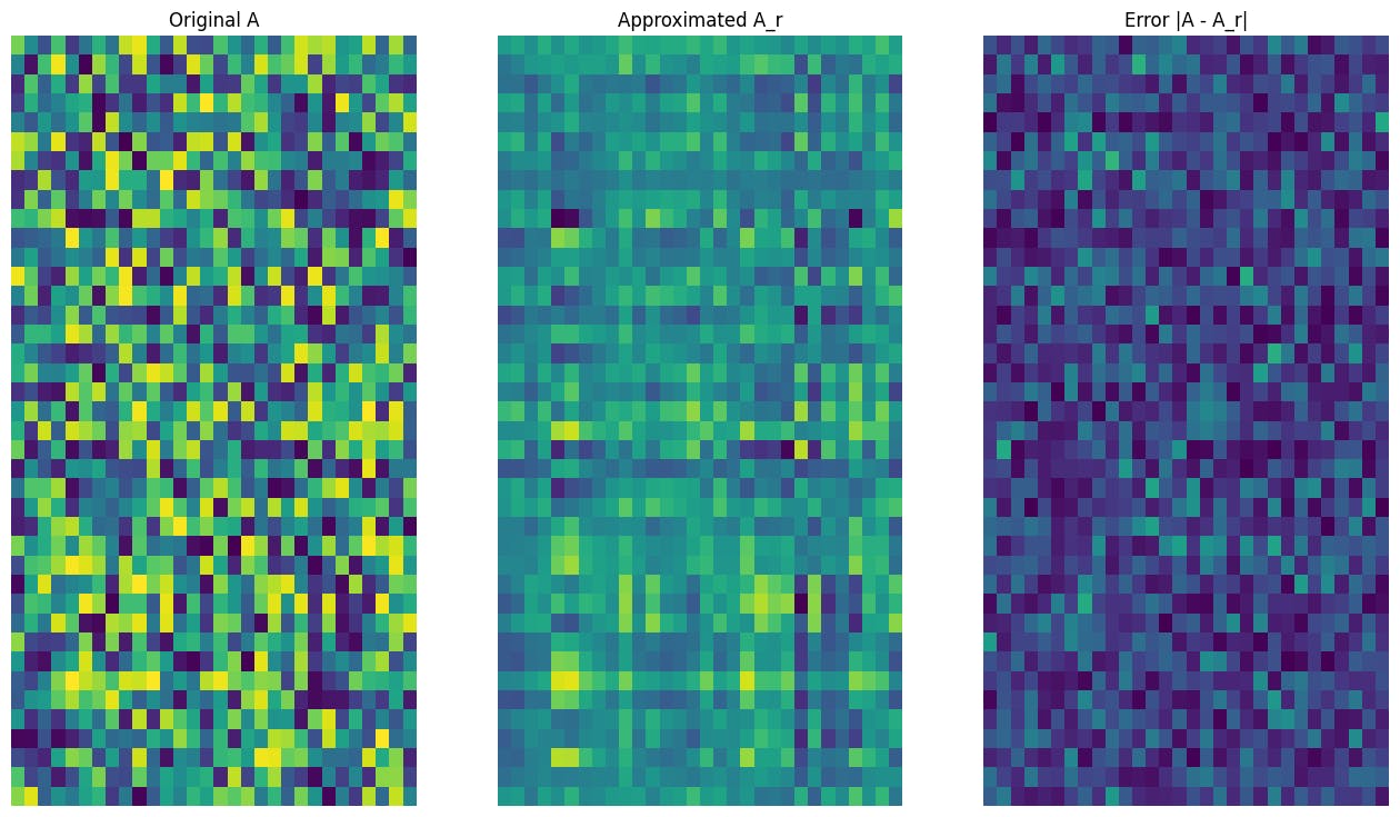
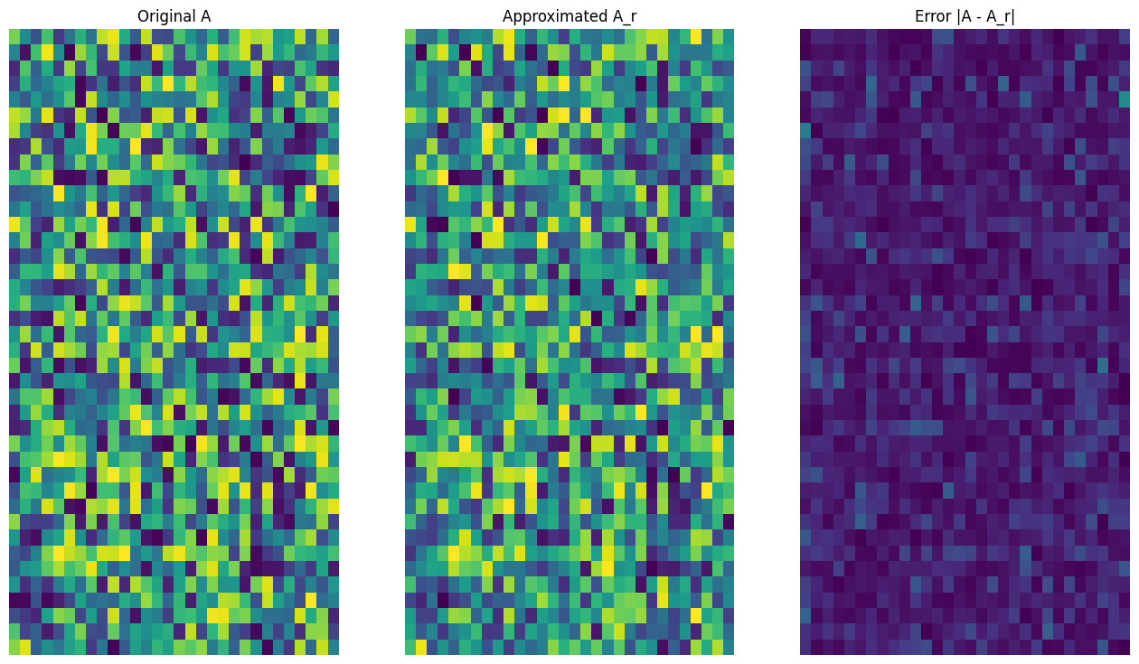
Начните с написания функции, чтобы вычислить аппроксимацию Rank-R данной матрицы. Эта процедура с низким уровнем приближения используется для сжатия изображения; Следовательно, также полезно вычислять размеры физических данных для каждого приближения. Для простоты предположим, что размер данных для аппроксимированной матрицы Rank-R равен общему количеству элементов, необходимых для вычисления приближения. Затем напишите функцию, чтобы визуализировать исходную матрицу, аппроксимацию его ранга, AR и матрица ошибок, | a-ar |.

def rank_r_approx(s, U, V, r, verbose=False):
  # Compute the matrices necessary for a rank-r approximation
  s_r, U_r, V_r = s[..., :r], U[..., :, :r], V[..., :, :r] # ... implies any number of extra batch axes
  # Compute the low-rank approximation and its size
  A_r = tf.einsum('...s,...us,...vs->...uv',s_r,U_r,V_r)
  A_r_size = tf.size(U_r) + tf.size(s_r) + tf.size(V_r)
  if verbose:
    print(f"Approximation Size: {A_r_size}")
  return A_r, A_r_size

def viz_approx(A, A_r):
  # Plot A, A_r, and A - A_r
  vmin, vmax = 0, tf.reduce_max(A)
  fig, ax = plt.subplots(1,3)
  mats = [A, A_r, abs(A - A_r)]
  titles = ['Original A', 'Approximated A_r', 'Error |A - A_r|']
  for i, (mat, title) in enumerate(zip(mats, titles)):
    ax[i].pcolormesh(mat, vmin=vmin, vmax=vmax)
    ax[i].set_title(title)
    ax[i].axis('off')

print(f"Original Size of A: {tf.size(A)}")
s, U, V = tf.linalg.svd(A)

Original Size of A: 1200

# Rank-15 approximation
A_15, A_15_size = rank_r_approx(s, U, V, 15, verbose = True)
viz_approx(A, A_15)

Approximation Size: 1065

# Rank-3 approximation
A_3, A_3_size = rank_r_approx(s, U, V, 3, verbose = True)
viz_approx(A, A_3)

Approximation Size: 213

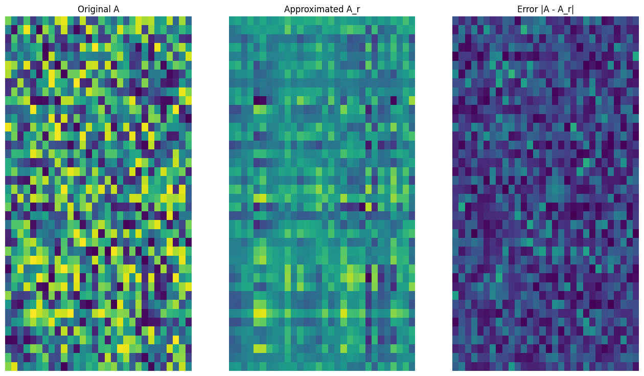
Как и ожидалось, использование более низких рангов приводит к менее тематическим приближениям. Тем не менее, качество этих низкодовольных приближений часто достаточно хороша в сценариях реального мира. Также обратите внимание, что основной целью низкого уровня приближения с SVD является снижение размерности данных, но не уменьшить пространство диска самих данных. Однако по мере того, как входные матрицы становятся более высокими измерениями, многие приближения с низким рейтингом также в конечном итоге получают выгоду от уменьшенного размера данных. Это преимущество в сокращении заключается в том, почему процесс применим для задач сжатия изображений.

Загрузка изображения

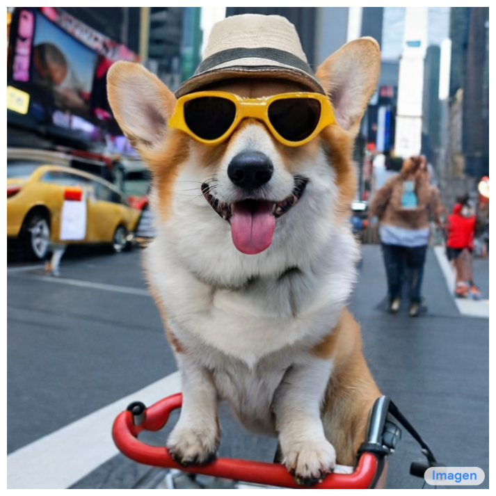
Следующее изображение доступно наВоображениедомашняя страница. Imagen-это модель диффузии текста до изображения, разработанная командой Google Research Brain Team. ИИ создал это изображение, основанное на подсказке: «Фотография собаки Корги, катающей на велосипеде на Таймс -сквер. На ней есть солнцезащитные очки и пляжная шляпа». Как это круто! Вы также можете изменить URL ниже на любую ссылку .jpg для загрузки на пользовательском изображении по выбору.

Начните с чтения и визуализации изображения. После прочтения файла JPEG Matplotlib выводит матрицу, I, формы (M × n × 3), которая представляет собой двухмерное изображение с 3 цветными каналами для красного, зеленого и синего соответственно.

img_link = "https://imagen.research.google/main_gallery_images/a-photo-of-a-corgi-dog-riding-a-bike-in-times-square.jpg"
img_path = requests.get(img_link, stream=True).raw
I = imread(img_path, 0)
print("Input Image Shape:", I.shape)

Input Image Shape: (1024, 1024, 3)

def show_img(I):
  # Display the image in matplotlib
  img = plt.imshow(I)
  plt.axis('off')
  return

show_img(I)

Алгоритм сжатия изображения

Теперь используйте SVD для вычисления низких приближений образца изображения. Напомним, что изображение имеет форму (1024 × 1024 × 3) и что теория SVD применяется только для двухмерных матриц. Это означает, что образцы изображения должны быть сопоставлены в 3 матрица одинакового размера, которые соответствуют каждому из 3 цветных каналов. Это можно сделать путем перемещения матрицы, чтобы иметь форму (3 × 1024 × 1024). Чтобы четко визуализировать ошибку аппроксимации, изменить значения RGB изображения от [0,255] до [0,1]. Не забудьте обрезать аппроксимированные значения, чтобы попасть в этот интервал, прежде чем визуализировать их. Аtf.clip_by_valueФункция полезна для этого.

def compress_image(I, r, verbose=False):
  # Compress an image with the SVD given a rank 
  I_size = tf.size(I)
  print(f"Original size of image: {I_size}")
  # Compute SVD of image
  I = tf.convert_to_tensor(I)/255
  I_batched = tf.transpose(I, [2, 0, 1]) # einops.rearrange(I, 'h w c -> c h w')
  s, U, V = tf.linalg.svd(I_batched)
  # Compute low-rank approximation of image across each RGB channel
  I_r, I_r_size = rank_r_approx(s, U, V, r)
  I_r = tf.transpose(I_r, [1, 2, 0]) # einops.rearrange(I_r, 'c h w -> h w c')
  I_r_prop = (I_r_size / I_size)
  if verbose:
    # Display compressed image and attributes
    print(f"Number of singular values used in compression: {r}")
    print(f"Compressed image size: {I_r_size}")
    print(f"Proportion of original size: {I_r_prop:.3f}")
    ax_1 = plt.subplot(1,2,1)
    show_img(tf.clip_by_value(I_r,0.,1.))
    ax_1.set_title("Approximated image")
    ax_2 = plt.subplot(1,2,2)
    show_img(tf.clip_by_value(0.5+abs(I-I_r),0.,1.))
    ax_2.set_title("Error")
  return I_r, I_r_prop

Теперь вычислите приближения Rank-R для следующих рангов: 100, 50, 10

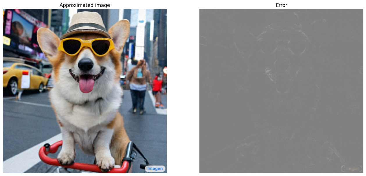
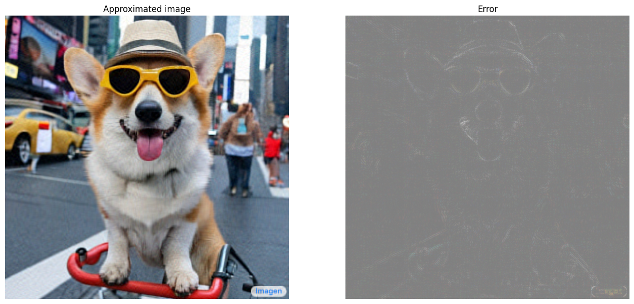
I_100, I_100_prop = compress_image(I, 100, verbose=True)

Original size of image: 3145728
Number of singular values used in compression: 100
Compressed image size: 614700
Proportion of original size: 0.195

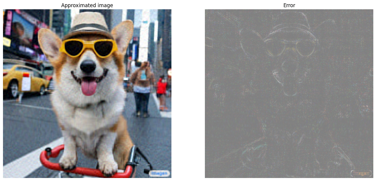
I_50, I_50_prop = compress_image(I, 50, verbose=True)

Original size of image: 3145728
Number of singular values used in compression: 50
Compressed image size: 307350
Proportion of original size: 0.098

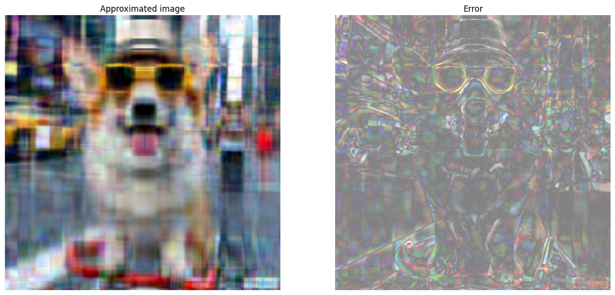
I_10, I_10_prop = compress_image(I, 10, verbose=True)

Original size of image: 3145728
Number of singular values used in compression: 10
Compressed image size: 61470
Proportion of original size: 0.020

Оценка приближения

Существует множество интересных методов для измерения эффективности и имеет больший контроль над матричными приближениями.

Коэффициент сжатия против ранга

Для каждого из вышеупомянутых приближений наблюдайте, как меняются размеры данных с рангом.

plt.figure(figsize=(11,6))
plt.plot([100, 50, 10], [I_100_prop, I_50_prop, I_10_prop])
plt.xlabel("Rank")
plt.ylabel("Proportion of original image size")
plt.title("Compression factor vs rank");

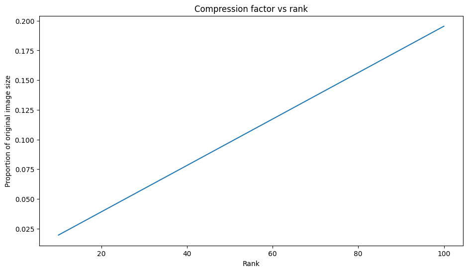
Основываясь на этом графике, существует линейная связь между аппроксимированным коэффициентом сжатия изображения и его рангом. Чтобы исследовать это, напомним, что размер данных аппроксимированной матрицы, AR, определяется как общее количество элементов, необходимых для ее вычисления. Следующие уравнения могут быть использованы для поиска взаимосвязи между коэффициентом сжатия и рангом:

x = (m × r)+r+(r × n) = r × (m+n+1)

c = xy = r × (m+n+1) m × n

где

• X: размер AR
• Y: размер а
• C = XY: коэффициент сжатия
• R: ранга приближения
• M и N: размеры строк и столбца

Чтобы найти ранг, r, который необходим для сжатия изображения к желаемому фактору, C, вышеупомянутое уравнение может быть перестановлено для решения для R:

r = ⌊c × m × nm+n+1⌋

Обратите внимание, что эта формула не зависит от размера цветового канала, поскольку каждое из приближений RGB не влияет друг на друга. Теперь напишите функцию для сжатия входного изображения с учетом желаемого коэффициента сжатия.

def compress_image_with_factor(I, compression_factor, verbose=False):
  # Returns a compressed image based on a desired compression factor
  m,n,o = I.shape
  r = int((compression_factor * m * n)/(m + n + 1))
  I_r, I_r_prop = compress_image(I, r, verbose=verbose)
  return I_r

Сжатие изображения до 15% от исходного размера.

compression_factor = 0.15
I_r_img = compress_image_with_factor(I, compression_factor, verbose=True)

Original size of image: 3145728
Number of singular values used in compression: 76
Compressed image size: 467172
Proportion of original size: 0.149

Кумулятивная сумма единственных значений

Совокупная сумма сингулярных значений может быть полезным показателем для количества энергии, захваченной приближением Rank-R. Визуализируйте усредненную RGB кумулятивную долю сингулярных значений в образце изображения. Аtf.cumsumФункция может быть полезна для этого.

def viz_energy(I):
  # Visualize the energy captured based on rank
  # Computing SVD
  I = tf.convert_to_tensor(I)/255
  I_batched = tf.transpose(I, [2, 0, 1]) 
  s, U, V = tf.linalg.svd(I_batched)
  # Plotting average proportion across RGB channels 
  props_rgb = tf.map_fn(lambda x: tf.cumsum(x)/tf.reduce_sum(x), s)
  props_rgb_mean = tf.reduce_mean(props_rgb, axis=0)
  plt.figure(figsize=(11,6))
  plt.plot(range(len(I)), props_rgb_mean, color='k')
  plt.xlabel("Rank / singular value number")
  plt.ylabel("Cumulative proportion of singular values")
  plt.title("RGB-averaged proportion of energy captured by the first 'r' singular values")

viz_energy(I)

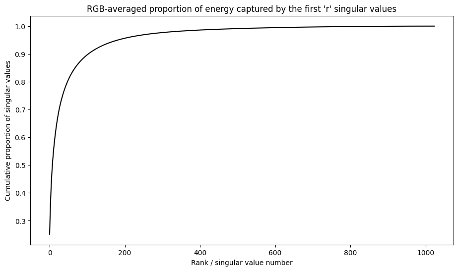
Похоже, что более 90% энергии на этом изображении фиксируется в первых 100 единственных значениях. Теперь напишите функцию для сжатия входного изображения с учетом желаемого коэффициента удержания энергии.

def compress_image_with_energy(I, energy_factor, verbose=False):
  # Returns a compressed image based on a desired energy factor
  # Computing SVD
  I_rescaled = tf.convert_to_tensor(I)/255
  I_batched = tf.transpose(I_rescaled, [2, 0, 1]) 
  s, U, V = tf.linalg.svd(I_batched)
  # Extracting singular values
  props_rgb = tf.map_fn(lambda x: tf.cumsum(x)/tf.reduce_sum(x), s)
  props_rgb_mean = tf.reduce_mean(props_rgb, axis=0)
  # Find closest r that corresponds to the energy factor
  r = tf.argmin(tf.abs(props_rgb_mean - energy_factor)) + 1
  actual_ef = props_rgb_mean[r]
  I_r, I_r_prop = compress_image(I, r, verbose=verbose)
  print(f"Proportion of energy captured by the first {r} singular values: {actual_ef:.3f}")
  return I_r

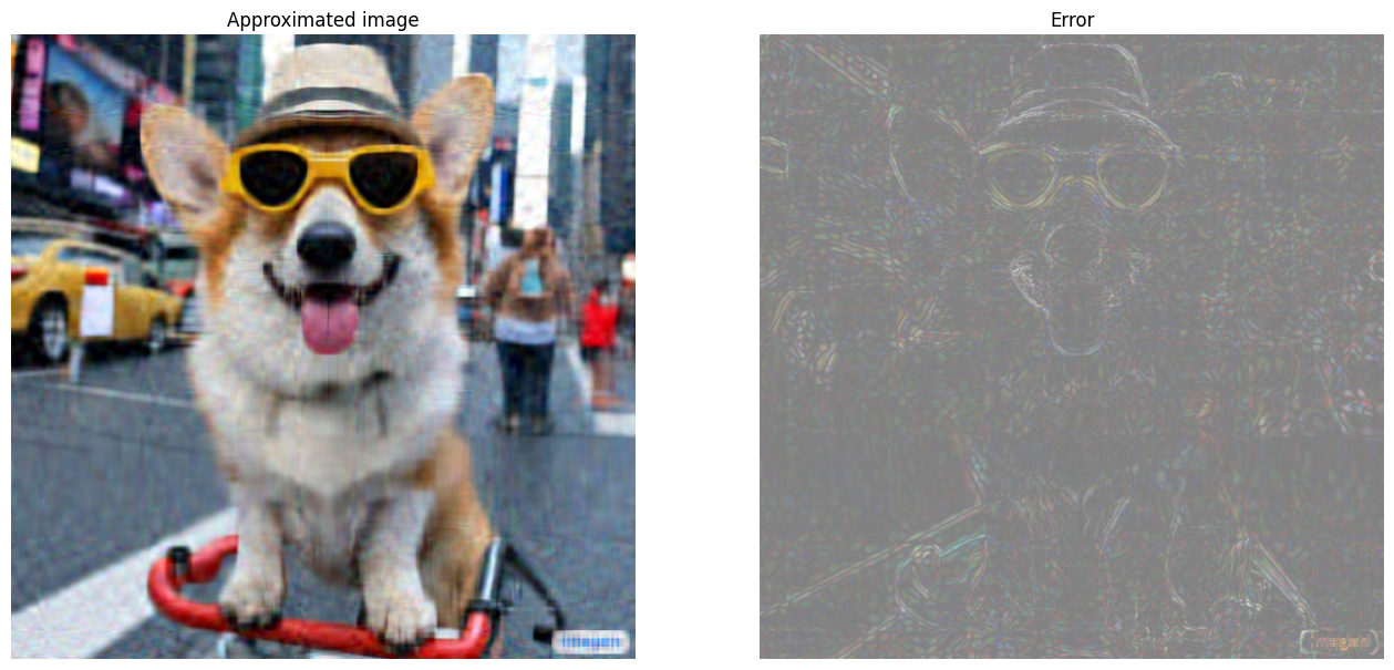
Сжатие изображения, чтобы сохранить 75% своей энергии.

energy_factor = 0.75
I_r_img = compress_image_with_energy(I, energy_factor, verbose=True)

Original size of image: 3145728
Number of singular values used in compression: 35
Compressed image size: 215145
Proportion of original size: 0.068
Proportion of energy captured by the first 35 singular values: 0.753

Ошибка и единственные значения

Существует также интересная связь между ошибкой аппроксимации и единственными значениями. Оказывается, что квадратная норма Фросениуса приближения равна сумме квадратов его единственных значений, которые были исключены:

|| a - ar || 2 = ∑i = r+1rσi2

Проверьте эту связь с приближением 10-го ранга примера матрицы в начале этого урока.

s, U, V = tf.linalg.svd(A)
A_10, A_10_size = rank_r_approx(s, U, V, 10)
squared_norm = tf.norm(A - A_10)**2
s_squared_sum = tf.reduce_sum(s[10:]**2)
print(f"Squared Frobenius norm: {squared_norm:.3f}")
print(f"Sum of squared singular values left out: {s_squared_sum:.3f}")

Squared Frobenius norm: 33.021
Sum of squared singular values left out: 33.021

Заключение

В этом записном книжке введены процесс реализации разложения единственного значения с помощью TensorFlow и применения его для написания алгоритма сжатия изображения. Вот еще несколько советов, которые могут помочь:

• АTensorflow Core APIможно использовать для различных высокопроизводительных вариантов использования научных вычислений.
• Чтобы узнать больше о линейных функциях алгебры Tensorflow, посетите документы дляМодуль ЛинальгаПолем
• SVD также может быть применен для построенияРекомендационные системыПолем

Для получения дополнительных примеров использования API -интерфейсов Core TensorFlow, ознакомьтесь сгидПолем Если вы хотите узнать больше о загрузке и подготовке данных, см. Учебные пособия наЗагрузка данных изображенияилиЗагрузка данных CSVПолем